| Version 13 (modified by klaurent, 2 years ago) (diff) |
|---|
ESM2025-N-cycle
This page is dedicated to the ESM2025 project (Earth System Models - European Project), especially for the N-cycle modelling. On this topic are working Marion Gehlen, Juliette Lathière, Didier Hauglustaine, Nicolas Vuichard and Karine Laurent.
Working Documents
- Notebooks :
- (22/04/20) 2 different notebooks are useful : Data_viewer and Analyse_3_sflx_NAT_dyn
- Data_viewer : To easily see a dataset. Interactive mode in order to change different variable at different time.
- Analyse_3_sflx_NAT_dyn : The 3 datasets (transcom, bouwman, piscidee=Pisces+orchidee) are loaded. Difference are computed (with Bouwman as a reference). Plots are made per month with same scale. Then, a seasonal analysis is done, calculating means/min/max of each dataset per month/year/season
- (22/04/20) 2 different notebooks are useful : Data_viewer and Analyse_3_sflx_NAT_dyn
- Emissions files :
- Bouwman : 360x180, created in 1999, Flux of agr waste burning, biofuel, biomass burning, deforestation, excreta, fossil fuel, industry, ocean, aquatic, soil
- Transcom : 360x180, created in 2015, total flux of N2O from OCN, PISCES and EDGAR
- Pisces (N2Oflx_OClim_CNRM-ESM2-1_piControl_r1i1p1f2_gn_185001-234912.nc), 362x294 (irregular grid), created in 2018, total flux of N2O for ocean
- Orchidee (ORCHIDEE_SH1_fN2O.nc), 720x360, created in 2022, total flux of N2O for land surfaces
- Bouwman Inventory :
- 846 N2O emission measurements in agricultural fields and 99 measurements for NO emissions
- The data set includes literature reference; location of the Measurement; climate; soil type, texture, organic C content, N content, drainage, and pH; residues left in the field; crop; fertilizer type; N application rate; method and timing of fertilizer application; NH4+ application rate (for organic fertilizers), N2O/NO emission/denitrification (expressed as total over the measurement period, as % of N rate, and as % of N rate accounting for control); measurement technique; length of measurement period; frequency of the measurements; and additional information, such as year/season of measurement, information on soil, crop or fertilizer management, specific characteristics of the fertilizer used, and specific weather events important for explaining the measured emissions.
- global gridded (1°x1° resolution) data bases of soil type, soil texture, NDVI (vegetation indices) and climate.
- global emission thus calculated is 6.8 Tg N2O-N y-1. The tropics (± 30° of the equator) contribute 5.4 Tg N2O-N y-1 and the emission from extra-tropical regions (poleward of 30°) is 1.4 Tg N2O-N y-1 .
- Transcom Inventory :
- "Emissions from natural soils (6–7 TgN yr −1 ) account for 60–70 % of global N2O emissions (Syakila and Kroeze, 2011; Zaehle et al., 2011). The remaining 30–40 % of emissions is from oceans (4.5 TgN yr −1 )"
- Five different inversion frameworks (chemistry transport model) : MOZART4 (2.5° × 1.88°), ACMt42167 (2.8° × 2.8°), TM3 (5.0° × 3.75°), TM5 (6.0° × 4.0°), LMDZ4 (3.75° × 2.5°).
- Data set from Orchidee O-CN, Pisces, edgar-4.1, gfed-2 and from different category (terrestrial biosphere, ocean, waste water, solid waste, solvents, fuel prod, ground transport, industry combustion, residential and other combustion, shipping, biomass burning)
Meeting Reports
On Wednesday, 1st June
On Wednesday, 18th May
In person with Juliette, Didier, Nicolas.
- Notebook Budget_inventories : total budget of N2O emissions (in tables), differences found between outputs INCASFLX and calculations in notebook (with mask, area and change units), different charts (by latitude, by land/ocean part, with histograms...)
Using the mask with fraction:
| FracMask? | - Output INCASFLX - | - Notebook computing - | ||||
| (Mt/yr) | Ocean | Land | Ratio O/L | Ocean | Land | Ratio O/L |
| Bouwman | 5.650486 | 11.83547 | 0.478 | 13.967 | 16.726 | 0.835 |
| 32.3% | 67.7% | 45.5% | 54.5% | |||
| Transcom | 6.634 | 16.614 | 0.399 | 8.879 | 14.421 | 0.616 |
| 28.5% | 71.5% | 38.1% | 61.9% | |||
| Piscidee | 6.432 | 7.107 | 0.905 | 6.579 | 6.989 | 0.941 |
| 47.5% | 52.5% | 48.5% | 51.5% | |||
Using the mask with 0/1 values:
| 0/1 Mask | - Output INCASFLX - | - Notebook computing - | ||||
| (Mt/yr) | Ocean | Land | Ratio O/L | Ocean | Land | Ratio O/L |
| Bouwman | 5.650486 | 11.83547 | 0.478 | 12.797 | 17.899 | 0.714 |
| 32.3% | 67.7% | 41.7% | 58.3% | |||
| Transcom | 6.634 | 16.614 | 0.399 | 8.118 | 15.184 | 0.535 |
| 28.5% | 71.5% | 34.8% | 65.2% | |||
| Piscidee | 6.432 | 7.107 | 0.905 | 6.174 | 7.395 | 0.834 |
| 47.5% | 52.5% | 45.5% | 54.5% | |||
Those differences can be explained by the different power that may exist between marine or continental fluxes at coasts notably. With mask, these two fluxes have the same importance so it changes total flux.
Values per latitudes:
| (Tg/yr) | 90-30S | 30S-0 | 0-30N | 30-90N | Total |
| Bouwman | 5.728 | 7.115 | 9.948 | 8.392 | 31.183 |
| Trancsom | 2.714 | 7.432 | 8.762 | 4.857 | 23.765 |
| Piscidee | 1.736 | 4.413 | 4.392 | 3.302 | 13.843 |
Calcul file by file: From Transcom (orchidee+pisces) : (no mask + not output of sflx) -> correspond to values of table 2 thompson part 1.
| - Output INCASFLX - | - Notebook computing - | |||||
| (Mt/yr) | Ocean | Land | Ratio O/L | Ocean | Land | Ratio O/L |
| Transcom | 6.634174 | 16.61481 | 0.399293 | 4.23125 | 10.59692 | 0.399291 |
Transcom is not a pre-industrial inventory, it's actual. So, it's better to work with piscidee inventory.
To DO
- Modify Bouwman run to take only 'oce' and 'soil' variables -> relaunch notebook to compare if it's better,
- Continue modification in INCA's code.
On Friday, 13th May
Informal with Didier.
Preparation to change INCA's code in Irene.
- Modify inca.card to take new NAT files and BBG from ciclad.
- Modify mksflx_p2p.F90 to put flx_n2o_ant to zero and add aflux terms.
- Modify sflx_inti.F90 to take into account BBG emissions.
- Modify set_ub_vals.F90 to rescale N2O flux (with parallel part and constant N2O flux at 285 ppb)
Launch different runs in order to check each step.
Next
- Change ANT in ciclad,
- Put flx_n2o_ant to 0,
- Erase the rescaling,
- Add N2O loss as an output...
On Wednesday, 4th May
In person with Juliette and Marion.
- Presentation of the Wiki page.
- Presentation of the two notebooks.
- Discussion on the different conceptions used in ocean and land communities (different grids, different units in the flux (mol/m2/s vs kg/m2/s)...).
On Analyse_3_sflx_NAT_dyn.ipynb, discussions on visualization with scale, calculation of the full emission on earth per year or per month.
To DO
- Make an analysis per month, per hemisphere, in order to get the total flux emissions for each inventory.
- Take information on where the inventories come from (especially Bouwman and Transcom).
- Draw tables which resume datas used, total emissions, models used in files...
- Compare native grid and regular grid for pisces.
- Compare values of each file used with outputs of INCASFLX.
- Compare total emissions on ocean and land with literature (ciais, ippc) and Bouwman and Trancsom inventories.
On Wednesday, 20th April
In person with Nicolas.
Discussion on:
- New page on Wiki/igcmg (this one !)
- Explanation of the created notebooks (Data_viewer and Analyse_3_sflx_NAT_dyn)
- Data_viewer : interactive ok but add choices/texts...
- Analyse_3_sflx_NAT_dyn : change the seasonal analysis made.
- Test with Nicolas' network to know about access to my notebooks.
- Speak about dods/orchidee to avoid downloading images on wiki.
Now, focus on N2O with long living time, but after, we can test on other compounds.
To DO
- Change colorbar with mean+/-std, add some texts on Notebooks and add units on charts
- Erase rescaling in Bouwman to have a better comparison
- Analyse the 3 datasets in a different way : global tables with sum per year, per region, per type (ocean/land) (watch out units)
- Give "procedure" and access to notebooks to all
- Compare with Auburn data (and Tian 2020)
- Look at Mendeley (or Zottero) for bibliography
Nicolas: Paths to have regional masks (from Transcom)
On Wednesday, 6th April
In Visio with Nicolas, Juliette, Didier, Marion.
Mainly, this meeting was to talk a bit more about the project and the work I(=Karine) can make before the training session (April 14th & 15th).
Discussion on:
- the first result made with INCAFLX and 3 different inventories,
- the planning we can set up (which kind of simulation...)
- the impact of N2O on chemistry (if everything is coupled),
- the certainty (or uncertainty) of inventories used (to determine an appropriate scaling),
- the work of Pierre for aquatic emissions (importance of river emissions),
Planning : Run simulation without chemistry and no rescaling, first for pre-industrial, then until now to see/understand the correction we can make on both period (a different correction for each period).
=> This have to be detailed and confirmed
Maybe run only 10 years to know where are sinks, determine some lifetime/seasonal cycle in order to calculate the scaling we may use.
Suggestions to work with the GES branch for the code (branch for coupled model with CO2, CH4 and N2O)
Meeting every 2 weeks same day, same time (ie, Wednesday at 10:00)
To DO
- Ask for writing a Wiki page on IGCMG
- Log on JupyterHub?
- Make an "experiment plan" for future simulations
- Analyse the results that I've already (seasonal analyses, comparison between inventories with Bouwman as a reference, recap origin/grid resolution...)
- Show the aquatic variable of Bouwman (and maybe some others)
Didier : emissions file for pre-industrial fires to be send to Karine
Bibliography
Attachments (17)
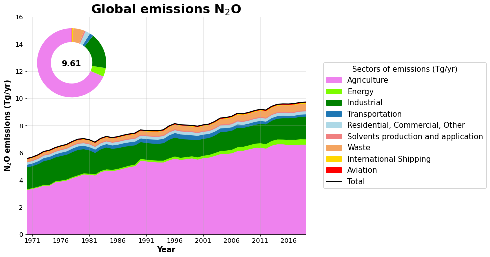
- N2O_emissions_CEDS.png (55.3 KB) - added by klaurent 23 months ago.
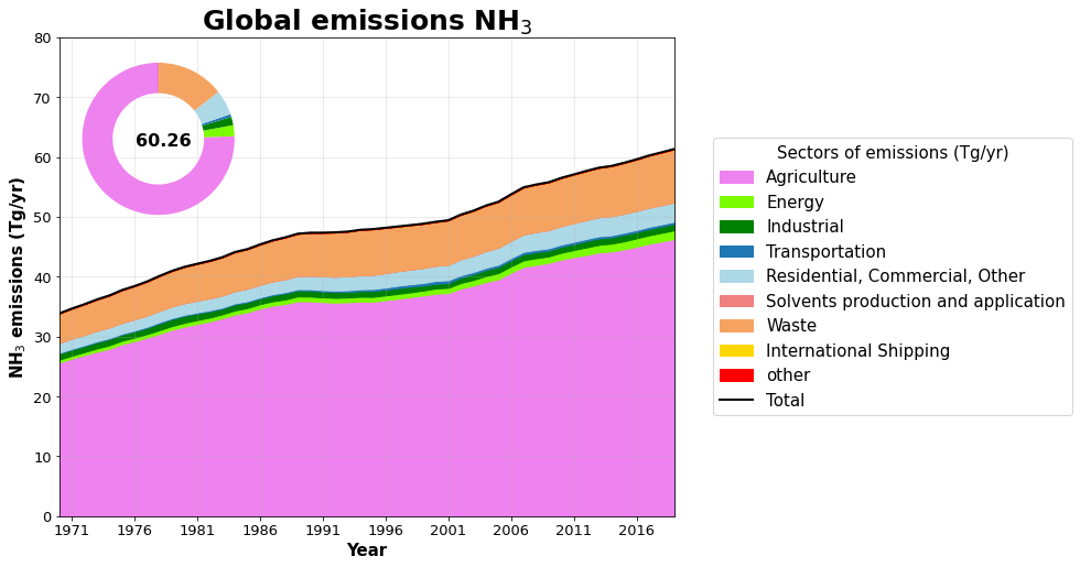
- NH3_emissions_CEDS.png (51.4 KB) - added by klaurent 23 months ago.
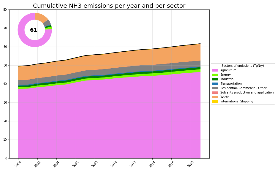
- NH3_CEDS_supplementary.png (71.6 KB) - added by klaurent 23 months ago.
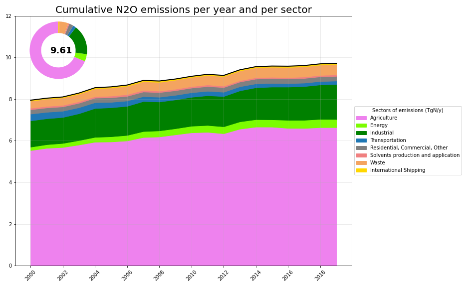
- N2O_CEDS_supplementary.png (78.3 KB) - added by klaurent 23 months ago.
- meeting_220824.pdf (464.2 KB) - added by klaurent 20 months ago.
- N2O_CEDS_supplementary_avion.png (77.8 KB) - added by klaurent 20 months ago.
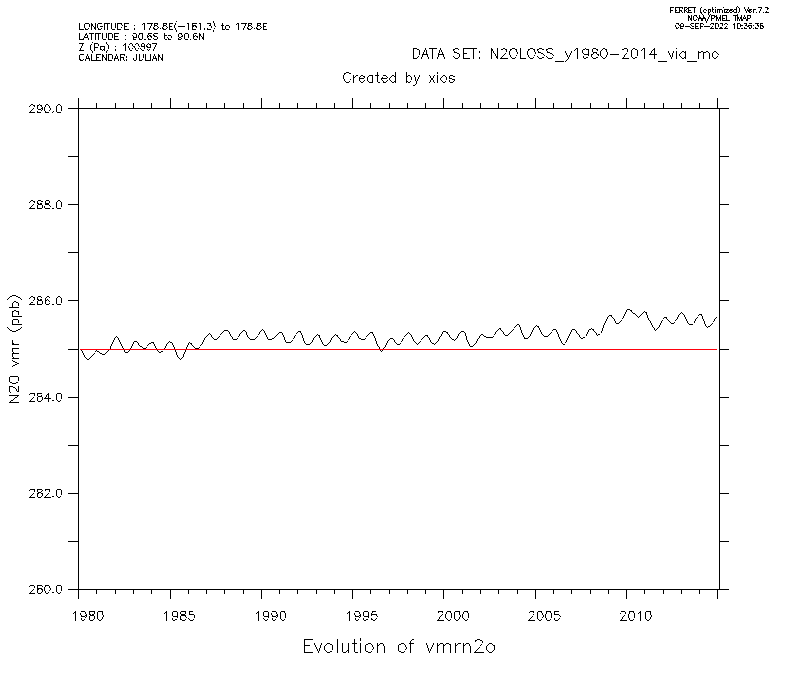
- ev_pi_vmr.png (10.2 KB) - added by klaurent 20 months ago.
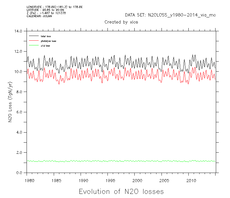
- ev_pi_loss.png (13.5 KB) - added by klaurent 20 months ago.
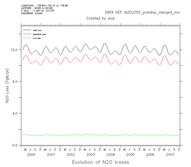
- loss_prstday_2000.png (9.9 KB) - added by klaurent 20 months ago.
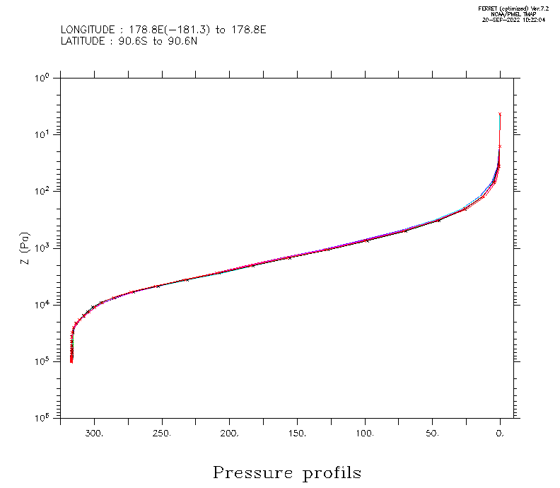
- vertical_profil_prstday_2000.png (22.0 KB) - added by klaurent 20 months ago.
- c1-vertical_profil_prstdayL.png (10.8 KB) - added by klaurent 19 months ago.
- c2-concentration_prstdayL.png (10.5 KB) - added by klaurent 19 months ago.
- c3-loss_prstday.png (12.2 KB) - added by klaurent 19 months ago.
- c4-burden_prstday.png (11.9 KB) - added by klaurent 19 months ago.
- a1-emissionsNAT.png (45.0 KB) - added by klaurent 19 months ago.
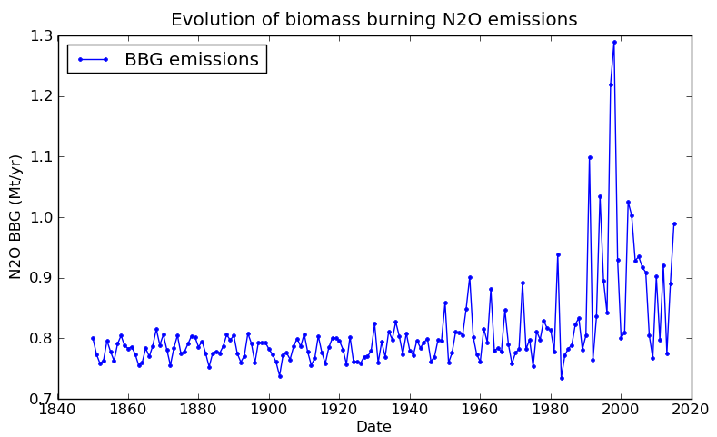
- a3-emissionsBBG.png (48.0 KB) - added by klaurent 19 months ago.
- a4-emissionsANT.png (42.8 KB) - added by klaurent 19 months ago.
Download all attachments as: .zip