Subgrid Scale Physics

The primitive equations describe the behaviour of a geophysical fluid at space and time scales larger than a few kilometres in the horizontal, a few meters in the vertical and a few minutes. They are usually solved at larger scales: the specified grid spacing and time step of the numerical model. The effects of smaller scale motions (coming from the advective terms in the Navier-Stokes equations) must be represented entirely in terms of large-scale patterns to close the equations. These effects appear in the equations as the divergence of turbulent fluxes ($i.e.$ fluxes associated with the mean correlation of small scale perturbations). Assuming a turbulent closure hypothesis is equivalent to choose a formulation for these fluxes. It is usually called the subgrid scale physics. It must be emphasized that this is the weakest part of the primitive equations, but also one of the most important for long-term simulations as small scale processes in fine balance the surface input of kinetic energy and heat.

The control exerted by gravity on the flow induces a strong anisotropy between the lateral and vertical motions. Therefore subgrid-scale physics D $^{\vect{U}}$, $D^{S}$ and $D^{T}$ in (2.1a), (2.1d) and (2.1e) are divided into a lateral part D $^{l \vect{U}}$, $D^{lS}$ and $D^{lT}$ and a vertical part D$^{vU}$, $D^{vS}$ and $D^{vT}$. The formulation of these terms and their underlying physics are briefly discussed in the next two subsections.

Vertical Subgrid Scale Physics

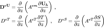
The model resolution is always larger than the scale at which the major sources of vertical turbulence occur (shear instability, internal wave breaking...). Turbulent motions are thus never explicitly solved, even partially, but always parameterized. The vertical turbulent fluxes are assumed to depend linearly on the gradients of large-scale quantities (for example, the turbulent heat flux is given by $\overline{T'w'}=-A^{vT} \partial_z \overline T$, where $A^{vT}$ is an eddy coefficient). This formulation is analogous to that of molecular diffusion and dissipation. This is quite clearly a necessary compromise: considering only the molecular viscosity acting on large scale severely underestimates the role of turbulent diffusion and dissipation, while an accurate consideration of the details of turbulent motions is simply impractical. The resulting vertical momentum and tracer diffusive operators are of second order:

$$\begin{split}{\vect{D}}^{v \vect{U}} &=\frac{\partial }{\part... ...left( {A^{vT}\frac{\partial S}{\partial z}} \right) \end{split}$$ (2.27)

where $A^{vm}$ and $A^{vT}$ are the vertical eddy viscosity and diffusivity coefficients, respectively. At the sea surface and at the bottom, turbulent fluxes of momentum, heat and salt must be specified (see Chap. 7 and 10 and §5.5). All the vertical physics is embedded in the specification of the eddy coefficients. They can be assumed to be either constant, or function of the local fluid properties ($e.g.$ Richardson number, Brunt-Vaisälä frequency...), or computed from a turbulent closure model. The choices available in NEMO are discussed in §10).

Formulation of the Lateral Diffusive and Viscous Operators

Lateral turbulence can be roughly divided into a mesoscale turbulence associated with eddies (which can be solved explicitly if the resolution is sufficient since their underlying physics are included in the primitive equations), and a sub mesoscale turbulence which is never explicitly solved even partially, but always parameterized. The formulation of lateral eddy fluxes depends on whether the mesoscale is below or above the grid-spacing ($i.e.$ the model is eddy-resolving or not).

In non-eddy-resolving configurations, the closure is similar to that used for the vertical physics. The lateral turbulent fluxes are assumed to depend linearly on the lateral gradients of large-scale quantities. The resulting lateral diffusive and dissipative operators are of second order. Observations show that lateral mixing induced by mesoscale turbulence tends to be along isopycnal surfaces (or more precisely neutral surfaces McDougall [1987]) rather than across them. As the slope of neutral surfaces is small in the ocean, a common approximation is to assume that the `lateral' direction is the horizontal, $i.e.$ the lateral mixing is performed along geopotential surfaces. This leads to a geopotential second order operator for lateral subgrid scale physics. This assumption can be relaxed: the eddy-induced turbulent fluxes can be better approached by assuming that they depend linearly on the gradients of large-scale quantities computed along neutral surfaces. In such a case, the diffusive operator is an isoneutral second order operator and it has components in the three space directions. However, both horizontal and isoneutral operators have no effect on mean ($i.e.$ large scale) potential energy whereas potential energy is a main source of turbulence (through baroclinic instabilities). Gent and Mcwilliams [1990] have proposed a parameterisation of mesoscale eddy-induced turbulence which associates an eddy-induced velocity to the isoneutral diffusion. Its mean effect is to reduce the mean potential energy of the ocean. This leads to a formulation of lateral subgrid-scale physics made up of an isoneutral second order operator and an eddy induced advective part. In all these lateral diffusive formulations, the specification of the lateral eddy coefficients remains the problematic point as there is no really satisfactory formulation of these coefficients as a function of large-scale features.

In eddy-resolving configurations, a second order operator can be used, but usually the more scale selective biharmonic operator is preferred as the grid-spacing is usually not small enough compared to the scale of the eddies. The role devoted to the subgrid-scale physics is to dissipate the energy that cascades toward the grid scale and thus to ensure the stability of the model while not interfering with the resolved mesoscale activity. Another approach is becoming more and more popular: instead of specifying explicitly a sub-grid scale term in the momentum and tracer time evolution equations, one uses a advective scheme which is diffusive enough to maintain the model stability. It must be emphasised that then, all the sub-grid scale physics is included in the formulation of the advection scheme.

All these parameterisations of subgrid scale physics have advantages and drawbacks. There are not all available in NEMO. In the $z$-coordinate formulation, five options are offered for active tracers (temperature and salinity): second order geopotential operator, second order isoneutral operator, Gent and Mcwilliams [1990] parameterisation, fourth order geopotential operator, and various slightly diffusive advection schemes. The same options are available for momentum, except Gent and Mcwilliams [1990] parameterisation which only involves tracers. In the $s$-coordinate formulation, additional options are offered for tracers: second order operator acting along $s-$surfaces, and for momentum: fourth order operator acting along $s-$surfaces (see §9).

Lateral Laplacian tracer diffusive operator

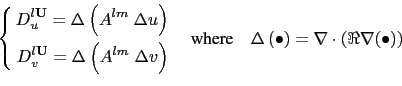
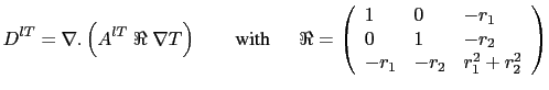
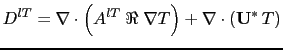
The lateral Laplacian tracer diffusive operator is defined by (see Appendix B):

$$D^{lT}=\nabla {\rm {\bf .}}\left( {A^{lT}\;\Re \;\nabla T} \right... ..._1 } \hfill & {-r_2 } \hfill & {r_1 ^2+r_2 ^2} \hfill \\ \end{array} }} \right)$$ (2.28)

where $r_1 \;$and$\;r_2$ are the slopes between the surface along which the diffusive operator acts and the model level ($e. g.$ $z$- or $s$-surfaces). Note that the formulation (2.35) is exact for the rotation between geopotential and $s$-surfaces, while it is only an approximation for the rotation between isoneutral and $z$- or $s$-surfaces. Indeed, in the latter case, two assumptions are made to simplify (2.35) [Cox, 1987]. First, the horizontal contribution of the dianeutral mixing is neglected since the ratio between iso and dia-neutral diffusive coefficients is known to be several orders of magnitude smaller than unity. Second, the two isoneutral directions of diffusion are assumed to be independent since the slopes are generally less than $10^{-2}$ in the ocean (see Appendix B).

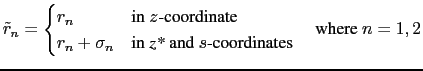
For iso-level diffusion, $r_1$ and $r_2$ are zero. $\Re$ reduces to the identity in the horizontal direction, no rotation is applied.

For geopotential diffusion, $r_1$ and $r_2$ are the slopes between the geopotential and computational surfaces: they are equal to $\sigma _1$ and $\sigma _2$, respectively (see (2.22) ).

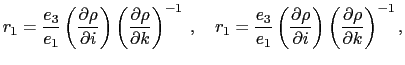
For isoneutral diffusion $r_1$ and $r_2$ are the slopes between the isoneutral and computational surfaces. Therefore, they are different quantities, but have similar expressions in $z$- and $s$-coordinates. In $z$-coordinates:

$$r_1 =\frac{e_3 }{e_1 } \left( {\frac{\partial \rho }{\partial i}}... ...}{\partial i}} \right) \left( {\frac{\partial \rho }{\partial k}} \right)^{-1},$$ (2.29)

while in $s$-coordinates $\partial/\partial k$ is replaced by $\partial/\partial s$.

Eddy induced velocity

When the eddy induced velocity parametrisation (eiv) [Gent and Mcwilliams, 1990] is used, an additional tracer advection is introduced in combination with the isoneutral diffusion of tracers:

$$D^{lT}=\nabla \cdot \left( {A^{lT}\;\Re \;\nabla T} \right) +\nabla \cdot \left( {{\vect{U}}^\ast \,T} \right)$$ (2.30)

where ${\vect{U}}^\ast =\left( {u^\ast ,v^\ast ,w^\ast } \right)$ is a non-divergent, eddy-induced transport velocity. This velocity field is defined by:

$$\begin{split}u^\ast &= +\frac{1}{e_3 }\frac{\partial }{\parti... ...\left( {A^{eiv}\;e_1\,\tilde{r}_2 } \right) \right] \end{split}$$ (2.31)

where $A^{eiv}$ is the eddy induced velocity coefficient (or equivalently the isoneutral thickness diffusivity coefficient), and $\tilde{r}_1$ and $\tilde{r}_2$ are the slopes between isoneutral and geopotential surfaces. Their values are thus independent of the vertical coordinate, but their expression depends on the coordinate:

$$\tilde{r}_n = \begin{cases}r_n & \text{in $z$-coordinate} \\ r_n ... ...\text{in \textit{z*} and $s$-coordinates} \end{cases} \quad \text{where } n=1,2$$ (2.32)

The normal component of the eddy induced velocity is zero at all the boundaries. This can be achieved in a model by tapering either the eddy coefficient or the slopes to zero in the vicinity of the boundaries. The latter strategy is used in NEMO (cf. Chap. 9).

Lateral bilaplacian tracer diffusive operator

The lateral bilaplacian tracer diffusive operator is defined by:

$$D^{lT}=\Delta \left( {A^{lT}\;\Delta T} \right) \ D^{lT}=\Delta \left( {A^{lT}\;\Delta T} \right)$$ (2.33)

It is the second order operator given by (2.35) applied twice with the eddy diffusion coefficient correctly placed.

Lateral Laplacian momentum diffusive operator

The Laplacian momentum diffusive operator along $z$- or $s$-surfaces is found by applying (2.7e) to the horizontal velocity vector (see Appendix B):

$$\begin{split}{\rm {\bf D}}^{l{\rm {\bf U}}} &= \quad \ \nabla _... ...e_3 \zeta} \right)}{\partial i} \end{aligned} \right) \end{split}$$

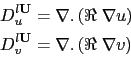
Such a formulation ensures a complete separation between the vorticity and horizontal divergence fields (see Appendix C). Unfortunately, it is not available for geopotential diffusion in $s-$coordinates and for isoneutral diffusion in both $z$- and $s$-coordinates ($i.e.$ when a rotation is required). In these two cases, the $u$ and $v-$fields are considered as independent scalar fields, so that the diffusive operator is given by:

$$\begin{split}D_u^{l{\rm {\bf U}}} &= \nabla .\left( {\Re \;\n... ...\bf U}}} &= \nabla .\left( {\Re \;\nabla v} \right) \end{split}$$ (2.35)

where $\Re$ is given by (2.35). It is the same expression as those used for diffusive operator on tracers. It must be emphasised that such a formulation is only exact in a Cartesian coordinate system, $i.e.$ on a $f-$ or $\beta-$plane, not on the sphere. It is also a very good approximation in vicinity of the Equator in a geographical coordinate system [Lengaigne et al., 2003].

lateral bilaplacian momentum diffusive operator

As for tracers, the fourth order momentum diffusive operator along $z$ or $s$-surfaces is a re-entering second order operator (2.41) or (2.41) with the eddy viscosity coefficient correctly placed:

geopotential diffusion in $z$-coordinate:

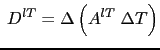
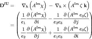
$$\begin{split}{\rm {\bf D}}^{l{\rm {\bf U}}} &=\nabla _h \left... ...\zeta \;{\rm {\bf k}}} \right)} \right]\;} \right\} \end{split}$$ (2.36)

geopotential diffusion in $s$-coordinate:

$$\left\{ \begin{aligned}D_u^{l{\rm {\bf U}}} =\Delta \left( {A^{... ...\bullet \right) = \nabla \cdot \left( \Re \nabla(\bullet) \right)$$