Next: Accuracy and Reproducibility (lib_fortran.F90) Up: Miscellaneous Topics Previous: Sub-Domain Functionality (jpizoom, jpjzoom) Contents Index
!-----------------------------------------------------------------------
&namdom        !   space and time domain (bathymetry, mesh, timestep)
!-----------------------------------------------------------------------
   nn_bathy    =    1      !  compute (=0) or read (=1) the bathymetry file
   rn_bathy    =    0.     !  value of the bathymetry. if (=0) bottom flat at jpkm1
   nn_closea   =    0      !  remove (=0) or keep (=1) closed seas and lakes (ORCA)
   nn_msh      =    1      !  create (=1) a mesh file or not (=0)
   rn_hmin     =   -3.     !  min depth of the ocean (>0) or min number of ocean level (<0)
   rn_e3zps_min=   20.     !  partial step thickness is set larger than the minimum of
   rn_e3zps_rat=    0.1    !  rn_e3zps_min and rn_e3zps_rat*e3t, with 0<rn_e3zps_rat<1
                           !
   rn_rdt      = 5760.     !  time step for the dynamics (and tracer if nn_acc=0)
   rn_atfp     =    0.1    !  asselin time filter parameter
   nn_acc      =    0      !  acceleration of convergence : =1      used, rdt < rdttra(k)
                                 !                          =0, not used, rdt = rdttra
   rn_rdtmin   = 28800.          !  minimum time step on tracers (used if nn_acc=1)
   rn_rdtmax   = 28800.          !  maximum time step on tracers (used if nn_acc=1)
   rn_rdth     =  800.           !  depth variation of tracer time step  (used if nn_acc=1)
   ln_crs      = .false.      !  Logical switch for coarsening module
   jphgr_msh   =       0               !  type of horizontal mesh
                                       !  = 0 curvilinear coordinate on the sphere read in coordinate.nc
                                       !  = 1 geographical mesh on the sphere with regular grid-spacing
                                       !  = 2 f-plane with regular grid-spacing
                                       !  = 3 beta-plane with regular grid-spacing
                                       !  = 4 Mercator grid with T/U point at the equator
   ppglam0     =       0.0             !  longitude of first raw and column T-point (jphgr_msh = 1)
   ppgphi0     =     -35.0             ! latitude  of first raw and column T-point (jphgr_msh = 1)
   ppe1_deg    =       1.0             !  zonal      grid-spacing (degrees)
   ppe2_deg    =       0.5             !  meridional grid-spacing (degrees)
   ppe1_m      =    5000.0             !  zonal      grid-spacing (degrees)
   ppe2_m      =    5000.0             !  meridional grid-spacing (degrees)
   ppsur       =    -4762.96143546300  !  ORCA r4, r2 and r05 coefficients
   ppa0        =      255.58049070440  ! (default coefficients)
   ppa1        =      245.58132232490  !
   ppkth       =       21.43336197938  !
   ppacr       =        3.0            !
   ppdzmin     =       10.             !  Minimum vertical spacing
   pphmax      =     5000.             !  Maximum depth
   ldbletanh   =    .TRUE.             !  Use/do not use double tanf function for vertical coordinates
   ppa2        =      100.760928500000 !  Double tanh function parameters
   ppkth2      =       48.029893720000 !
   ppacr2      =       13.000000000000 !
/
Searching an equilibrium state with an global ocean model requires a very long time integration period (a few thousand years for a global model). Due to the size of the time step required for numerical stability (less than a few hours), this usually requires a large elapsed time. In order to overcome this problem, Bryan [1984] introduces a technique that is intended to accelerate the spin up to equilibrium. It uses a larger time step in the tracer evolution equations than in the momentum evolution equations. It does not affect the equilibrium solution but modifies the trajectory to reach it.
Options are defined through the namdom namelist variables.
The acceleration of convergence option is used when nn_acc=1. In that case,
![]() is the time step of dynamics while
is the time step of dynamics while
![]() is the
tracer time-step. the former is set from the rn_rdt namelist parameter while the latter
is computed using a hyperbolic tangent profile and the following namelist parameters :
rn_rdtmin, rn_rdtmax and rn_rdth. Those three parameters correspond
to the surface value the deep ocean value and the depth at which the transition occurs, respectively.
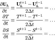
The set of prognostic equations to solve becomes:
is the
tracer time-step. the former is set from the rn_rdt namelist parameter while the latter
is computed using a hyperbolic tangent profile and the following namelist parameters :
rn_rdtmin, rn_rdtmax and rn_rdth. Those three parameters correspond
to the surface value the deep ocean value and the depth at which the transition occurs, respectively.
The set of prognostic equations to solve becomes:
Bryan [1984] has examined the consequences of this distorted physics.
Free waves have a slower phase speed, their meridional structure is slightly
modified, and the growth rate of baroclinically unstable waves is reduced
but with a wider range of instability. This technique is efficient for
searching for an equilibrium state in coarse resolution models. However its
application is not suitable for many oceanic problems: it cannot be used for
transient or time evolving problems (in particular, it is very questionable
to use this technique when there is a seasonal cycle in the forcing fields),
and it cannot be used in high-resolution models where baroclinically
unstable processes are important. Moreover, the vertical variation of
![]() implies that the heat and salt contents are no longer
conserved due to the vertical coupling of the ocean level through both
advection and diffusion. Therefore rn_rdtmin = rn_rdtmax should be
a more clever choice.
implies that the heat and salt contents are no longer
conserved due to the vertical coupling of the ocean level through both
advection and diffusion. Therefore rn_rdtmin = rn_rdtmax should be
a more clever choice.
Gurvan Madec and the NEMO Team
NEMO European Consortium2016-11-22