Next: Lateral/Vertical Momentum Diffusive Operators Up: Appendix B : Diffusive Previous: Horizontal/Vertical 2nd Order Tracer Contents Index
The iso/diapycnal diffusive tensor
![]() expressed in the (
expressed in the (![]() ,
,![]() ,
,![]() )
curvilinear coordinate system in which the equations of the ocean circulation model are
formulated, takes the following form [Redi, 1982]:
)
curvilinear coordinate system in which the equations of the ocean circulation model are
formulated, takes the following form [Redi, 1982]:
 |
In practice, isopycnal slopes are generally less than ![]() in the ocean, so
in the ocean, so
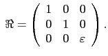
![]() can be simplified appreciably [Cox, 1987]:
can be simplified appreciably [Cox, 1987]:
Physically, the full tensor (B.3)
represents strong isoneutral diffusion on a plane parallel to the isoneutral
surface and weak dianeutral diffusion perpendicular to this plane.
However, the approximate `weak-slope' tensor (B.4a) represents strong
diffusion along the isoneutral surface, with weak
vertical diffusion - the principal axes of the tensor are no
longer orthogonal. This simplification also decouples
the (![]() ,
,![]() ) and (
) and (![]() ,
,![]() ) planes of the tensor. The weak-slope operator therefore takes the same
form, (B.4), as (B.2), the diffusion operator for geopotential
diffusion written in non-orthogonal
) planes of the tensor. The weak-slope operator therefore takes the same
form, (B.4), as (B.2), the diffusion operator for geopotential
diffusion written in non-orthogonal ![]() -coordinates. Written out
explicitly,
-coordinates. Written out
explicitly,
The isopycnal diffusion operator (B.4), (B.5) conserves tracer quantity and dissipates its square. The demonstration of the first property is trivial as (B.4) is the divergence of fluxes. Let us demonstrate the second one:
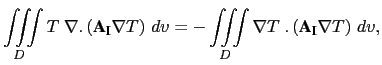 |
![\begin{subequations}\begin{align*}{\begin{array}{*{20}l} \nabla T\;.\left( {{\rm...
...ial k}\right) ^2\right] \\ & \geq 0 \end{array} } \end{align*}\end{subequations}](img3083.png?doc=NEMO) |
Because the weak-slope operator (B.4), (B.5) is decoupled
in the (![]() ,
,![]() ) and (
) and (![]() ,
,![]() ) planes, it may be transformed into
generalized
) planes, it may be transformed into
generalized ![]() -coordinates in the same way as (B.1) was transformed into
(B.2). The resulting operator then takes the simple form
-coordinates in the same way as (B.1) was transformed into
(B.2). The resulting operator then takes the simple form
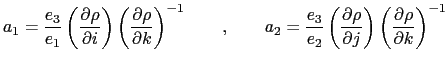
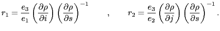
where (![]() ,
, ![]() ) are the isopycnal slopes in (
) are the isopycnal slopes in (
![]() ,
,
![]() ) directions, relative to
) directions, relative to ![]() -coordinate surfaces:
-coordinate surfaces:
 |
To prove (B.7) by direct re-expression of (B.5) is
straightforward, but laborious. An easier way is first to note (by reversing the
derivation of (B.2) from (B.1) ) that the
weak-slope operator may be exactly reexpressed in
non-orthogonal ![]() -coordinates as
-coordinates as
Note that the weak-slope approximation is only made in
transforming from the (rotated,orthogonal) isoneutral axes to the
non-orthogonal ![]() -coordinates. The further transformation
into
-coordinates. The further transformation
into ![]() -coordinates is exact, whatever the steepness of
the
-coordinates is exact, whatever the steepness of
the ![]() -surfaces, in the same way as the transformation of
horizontal/vertical Laplacian diffusion in
-surfaces, in the same way as the transformation of
horizontal/vertical Laplacian diffusion in ![]() -coordinates,
(B.1) onto
-coordinates,
(B.1) onto ![]() -coordinates is exact, however steep the
-coordinates is exact, however steep the ![]() -surfaces.
-surfaces.
Gurvan Madec and the NEMO Team
NEMO European Consortium2016-11-22
![$\displaystyle \textbf {A}_{\textbf I} = \frac{A^{lT}}{\left( {1+a_1 ^2+a_2 ^2} ...
... {-a_2 } \hfill & {\varepsilon +a_1 ^2+a_2 ^2} \hfill \\ \end{array} }} \right]$](img3067.png?doc=NEMO)
![$\displaystyle \begin{equation}{\textbf{A}_{\textbf{I}}} \approx A^{lT}\;\Re\;\t...
...t[ A^{lT} \;\Re \cdot \left. \nabla \right\vert _z T \right]. \\ \end{equation}$](img3075.png?doc=NEMO)
![\begin{multline}
D^T=\frac{1}{e_1 e_2 }\left\{
{\;\frac{\partial }{\partial i}...
...ight)}{e_3 }\frac{\partial T}{\partial k}} \right)} \right]}. \\
\end{multline}](img3081.png?doc=NEMO)
![$\displaystyle D^T = \left. \nabla \right\vert _s \cdot \left[ A^{lT} \;\Re \cdot \left. \nabla \right\vert _s T \right] \\ \;\;$](img3089.png?doc=NEMO) where
where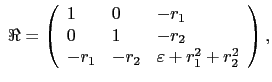
![$\displaystyle D^T = \left. \nabla \right\vert _\rho \cdot \left[ A^{lT} \;\Re \cdot \left. \nabla \right\vert _\rho T \right] \\ \;\;$](img3098.png?doc=NEMO) where
where