Next: Hydrostatic pressure gradient (dynhpg) Up: Ocean Dynamics (DYN) Previous: Coriolis and Advection: vector Contents Index
!-----------------------------------------------------------------------
&namdyn_adv    !   formulation of the momentum advection
!-----------------------------------------------------------------------
   ln_dynadv_vec = .true.  !  vector form (T) or flux form (F)
   nn_dynkeg     = 0       ! scheme for grad(KE): =0   C2  ;  =1   Hollingsworth correction
   ln_dynadv_cen2= .false. !  flux form - 2nd order centered scheme
   ln_dynadv_ubs = .false. !  flux form - 3rd order UBS      scheme
   ln_dynzad_zts = .false. !  Use (T) sub timestepping for vertical momentum advection
/
Options are defined through the namdyn_adv namelist variables.
In the flux form (as in the vector invariant form), the Coriolis and momentum
advection terms are evaluated using a leapfrog scheme, ![]() the velocity
appearing in their expressions is centred in time (now velocity). At the
lateral boundaries either free slip, no slip or partial slip boundary conditions
are applied following Chap.8.
the velocity
appearing in their expressions is centred in time (now velocity). At the
lateral boundaries either free slip, no slip or partial slip boundary conditions
are applied following Chap.8.
In flux form, the vorticity term reduces to a Coriolis term in which the Coriolis
parameter has been modified to account for the "metric" term. This altered
Coriolis parameter is thus discretised at ![]() -points. It is given by:
-points. It is given by:
Any of the (C.13), (6.6) and (C.15)
schemes can be used to compute the product of the Coriolis parameter and the
vorticity. However, the energy-conserving scheme (C.15) has
exclusively been used to date. This term is evaluated using a leapfrog scheme,
![]() the velocity is centred in time (now velocity).
the velocity is centred in time (now velocity).
The discrete expression of the advection term is given by :
Two advection schemes are available: a ![]() order centered finite
difference scheme, CEN2, or a
order centered finite
difference scheme, CEN2, or a ![]() order upstream biased scheme, UBS.
The latter is described in Shchepetkin and McWilliams [2005]. The schemes are
selected using the namelist logicals ln_dynadv_cen2 and ln_dynadv_ubs.
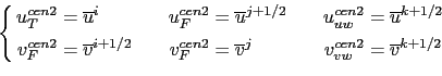
In flux form, the schemes differ by the choice of a space and time interpolation to
define the value of
order upstream biased scheme, UBS.
The latter is described in Shchepetkin and McWilliams [2005]. The schemes are
selected using the namelist logicals ln_dynadv_cen2 and ln_dynadv_ubs.
In flux form, the schemes differ by the choice of a space and time interpolation to
define the value of ![]() and
and ![]() at the centre of each face of
at the centre of each face of ![]() - and
- and ![]() -cells,
-cells,
![]() at the
at the ![]() -,
-, ![]() -, and
-, and ![]() -points for
-points for ![]() and at the
and at the ![]() -,
-, ![]() - and
- and
![]() -points for
-points for ![]() .
.
In the centered ![]() order formulation, the velocity is evaluated as the
mean of the two neighbouring points :
order formulation, the velocity is evaluated as the
mean of the two neighbouring points :
The scheme is non diffusive (i.e. conserves the kinetic energy) but dispersive
(![]() it may create false extrema). It is therefore notoriously noisy and must be
used in conjunction with an explicit diffusion operator to produce a sensible solution.
The associated time-stepping is performed using a leapfrog scheme in conjunction
with an Asselin time-filter, so
it may create false extrema). It is therefore notoriously noisy and must be
used in conjunction with an explicit diffusion operator to produce a sensible solution.
The associated time-stepping is performed using a leapfrog scheme in conjunction
with an Asselin time-filter, so ![]() and
and ![]() are the now velocities.
are the now velocities.
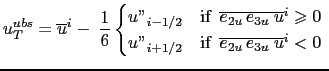
The UBS advection scheme is an upstream biased third order scheme based on
an upstream-biased parabolic interpolation. For example, the evaluation of
![]() is done as follows:
is done as follows:
The UBS scheme is not used in all directions. In the vertical, the centred ![]() order evaluation of the advection is preferred,
order evaluation of the advection is preferred, ![]()
![]() and
and
![]() in (6.16) are used. UBS is diffusive and is
associated with vertical mixing of momentum.
in (6.16) are used. UBS is diffusive and is
associated with vertical mixing of momentum.
For stability reasons, the first term in (6.17), which corresponds to a second order centred scheme, is evaluated using the now velocity (centred in time), while the second term, which is the diffusion part of the scheme, is evaluated using the before velocity (forward in time). This is discussed by Webb et al. [1998] in the context of the Quick advection scheme.
Note that the UBS and QUICK (Quadratic Upstream Interpolation for Convective Kinematics)
schemes only differ by one coefficient. Replacing ![]() by
by ![]() in
(6.17) leads to the QUICK advection scheme [Webb et al., 1998].
This option is not available through a namelist parameter, since the
in
(6.17) leads to the QUICK advection scheme [Webb et al., 1998].
This option is not available through a namelist parameter, since the ![]() coefficient
is hard coded. Nevertheless it is quite easy to make the substitution in the
dynadv_ubs.F90 module and obtain a QUICK scheme.
coefficient
is hard coded. Nevertheless it is quite easy to make the substitution in the
dynadv_ubs.F90 module and obtain a QUICK scheme.
Note also that in the current version of dynadv_ubs.F90, there is also the
possibility of using a ![]() order evaluation of the advective velocity as in
ROMS. This is an error and should be suppressed soon.
order evaluation of the advective velocity as in
ROMS. This is an error and should be suppressed soon.
Gurvan Madec and the NEMO Team
NEMO European Consortium2016-11-22
![\begin{multline}
f+\frac{1}{e_1 e_2 }\left( {v\frac{\partial e_2 }{\partial i} -...
...ne u ^{j+1/2}\delta _{j+1/2} \left[ {e_{1u} } \right] } \ \right)
\end{multline}](img1503.png?doc=NEMO)
![\begin{equation*}\left\{ \begin{aligned}\frac{1}{e_{1u}\,e_{2u}\,e_{3u}} \left( ...
...2w}\;w}^{j+1/2} \ v_{vw} \right] \right) \\ \end{aligned} \right.\end{equation*}](img1505.png?doc=NEMO)