Doc/Chap2 – Post_it

Context Navigation

Version 20 (modified by kolasinski, 16 years ago) (diff)
--

Chap.2 : File post_it.pro

General description and a first example

post_it.pro is the file in which you will work. It defines the in line commands which will be read by post_it so as to get the plot you want. For instance :

cmdline = [ $
; var             on   exp      grid  plt   timeave  date1   spec  disp   proj   out
  'sohtc300   1     2L24   T       xy   100y      1860     -       1       1        v', $

'lastline 0' ]

This means that you want the sohtc300 variable to be visualised from a netcdf file called '2L24_100y_1860_*_grid_T.nc' on a 2D plot 'xy'.
The result is the following picture (the quality is better in "ps" format than in "gif" format below).

As a consequence, the names of the netcdf files are standardized and follow this pattern :
'Experiment'_'Frequency'_'Date1'_'Date2'_'Grid Type'.nc

More details about the variables defined in 'post_it.pro'

Variable 'spec_base_list' defines where to find a specific database of files. It should begins with the name of the experiment (here all files beginning with 'CMAP_')
```
spec_base_list = [ $ 
 'CMAP = local:/home2/mkdlod/database/CORREL/', $
' ']
```

Variable 'data_base_list' defines also where to find by default all the databases ('ncdf_db'). Il also allows to define generic databases. For instance, 'MRI_db' defines all files beginning with 'MRI' : it can be 'MRI_', 'MRIoCTL', 'MRIo2X'...
```
data_base_list =  [ $
'ncdf_db = local:/home2/mkdlod/database/', $
'MRI_db = local:/home2/mkdlod/ERIC-LSCE/database/IPCC/',  $
' ']
```

Variable 'out_ps' defines where to find the postscripts files generated and puts them in the 'iodir' directory.
```
out_ps = homedir+'/Post_out/'
```

Variables 'prt_BW', 'prt_col', 'prt_tra' define the unix print command you want to use for printing postscripts files. This does not work at the moment in my case !!!!!!
```
prt_BW  = 'lpl'
prt_col = 'x4'
prt_tra = 'lprdgt'
```

Variable 'lp_opt'
```
lp_opt = ''
```

Variable 'ghost'
```
ghost = 'lpg'
```

Variable 'out_all' : if you want to override all the local 'out' options (each in line command has a specific 'out' option). For instance, you visualised 10 plots already and you want to print them all. Instead of setting all the individual in line 'out' options, you set 'out_all' to 'ps' once and for all. By default, it shoud be set to '-' to avoid to override local 'out' options.
```
out_all = '-'
```

Variable 'other_file' : Instead of using the file 'post_it.pro' to read the in line commands, you would like to use another file ('post_it.pro' might be too big). For this purpose, set the variable 'other_file' to the name of the other file. By default, it is set to '-', which means 'post_it.pro' has to be read. Pay attention to the fact that the structure of the other file is bit different from 'post_it.pro' since you should only find the 'cmdline2' variable (similar to 'cmdline' from 'post_it.pro') in it.
```
other_file = 'post_it2'
other_file = '-'
```

Variable 'cmdline' : In this very long variable, you set the plot you want to see or print. Please check the other example below :

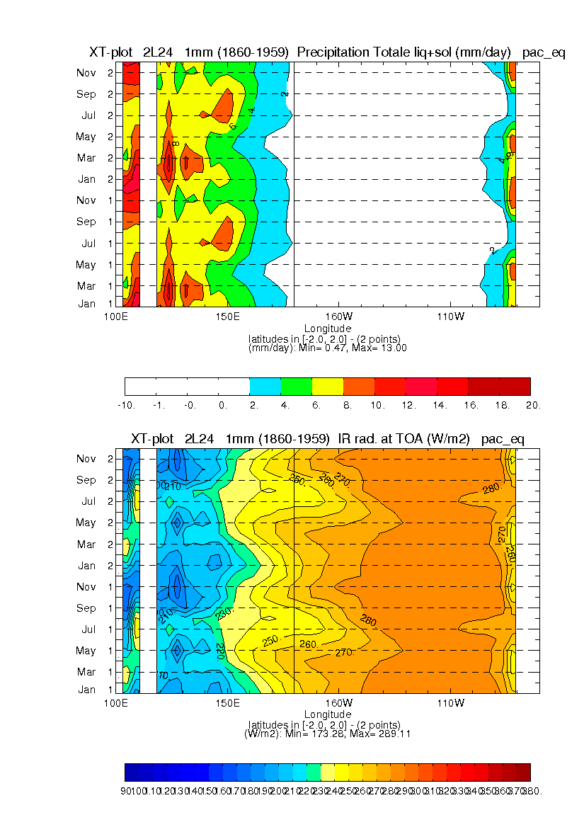
cmdline = [ $
; var        on   exp     grid  plt               timave   date1                spec                    disp   proj   out
  'precip   1   2L24  lmdzl  xt_pac_eq  1mm     01_1860-1959  12_1860-1959     2P     1        v', $
  'topl     0   2L24  lmdzl  xt_pac_eq  1mm     01_1860-1959  12_1860-1959     1       1        v', $

'lastline 0' ]

This in line command allows to see 2 plots on the same window ('Paysage' format). These are the seasonnal cycle of precipitation (called precip) and OLR (called topl) for the '2L24' experiment along the equator ('x' -> longitude, 't' -> time). The variable is averaged zonally on the box 'pac_eq' which is defined in 'domain_boxes.def' file. The grid type is 'lmdzl'. The file should contains 12 mean months from January to December and those mean months are carried out on 100 years from 1860 to 1959. The result is the following picture.

At the end of the 'post_it.pro' file, the program is launched through the following command :

def_work, data_base_list, out_ps, cmdline, out_all, other_file,  spec_base_list

Usage of command line ?

cmdline = [ $
; var        on   exp     grid  plt               timeave   date1                spec                    disp   proj   out
'lastline 0' ]

'var' : The name of the field is usually the long_name stored in the netcdf file. If you add '@@' at the beginning, it means that post_it will read 'fld_macros.def' to get the right macro to launch (for instance, compute the standard deviation of the sosstsst field through @@sosstdev)

; var : <name> of field
;         @@<name> for macro defined in Defaults/fld_macros.def
;         <name1>=f(<name2>) for scatter plot y=f(x) or
;         <name1>=f(next) to use next line as 'x' (uses time interval of name1)
;         <name>@s<sigma> to plot <name> on isopycnal <sigma>

  '@@sosstdev  1  CDT3   T      xyt   1m@t412  187001  196912  1     1   v', $

'on' : If you want to see a plot, set this variable to '1'. When you want several plots on the same window, you may hide one of these by setting 'on' to '2'. It will leave a blank space where the plot should have been drawn.

; on    : 0/1 (2 = empty window in multi-window plot)

  '@@sosstdev    1   CDT3   T      xyt   1m@t412  187001  196912  2x2     1   v', $
  '@@sotoxdev   2   CDT3   U      xyt   1m@t412  187001  196912  1     1   v', $
  '@@sotoxdev   0   CDT3   U      xyt   1m@t412  187001  196912  1     1   v', $
  '@@sotoydev   0   CDT3   V      xyt   1m@t412  187001  196912  1     1   v', $

'exp' : If you want to make a difference between 2 experiments, you 2 have options. This is the first one. Pay attention to the fact that the 2 files should have the same 'var' name, the same 'grid', the same 'timeave', the same 'plt', the same 'date1'...
```
; exp   : name of exp. For difference of 2 exp : <exp1>-<exp2>
;                                 For division of 2 exp : <exp1>/<exp2>

  'sozotaux     1   CD2-2L24  U     xt_pac_eq   1mm   01_1860-1959  12_1860-1959   2P   1  v', $
```

'grid' : The grid type defines the grids (regular or irregular like the ORCA grid) to read. For instance, post_it will read grids_ncpt62.nc which is stored in 'IDL/Defaults/Grids'. This grid is considered as regular (because you specified it in plt_def.pro in the variable 'nc_grid_list'). This file contains 3 variables : the land sea mask fraction, latitudes as a 1D variable and longitudes as a 1D variables. And post_it through saxo routines will build the grid with the help of those variables : gphit (eg latitudes), glamt (longitudes), tmask (masks on T-points), e1t (scale factor along x), e2t (scale factor along y) as 2D variables... Usually the atmospheric grids are regular. You can get easily the 'grids_...' files through the IPCC database with the variable 'sftlf' and build a new âgridâ. At the moment, only 2D field can be read from these grid. If the variable is stored in an irregular grid, things are a bit more complicated to build a new grid readable by post_it and saxo. You will need to build a file where the variables gphit, glamt, glamu, glamv, tmask... are already stored. For the moment, the ORCA grid (NEMO, IPSL) and the MICOM grid (BCM model, NERSC) can be read (even 3D fields). These grids are Arakawa C-type with T, U, V and F points.
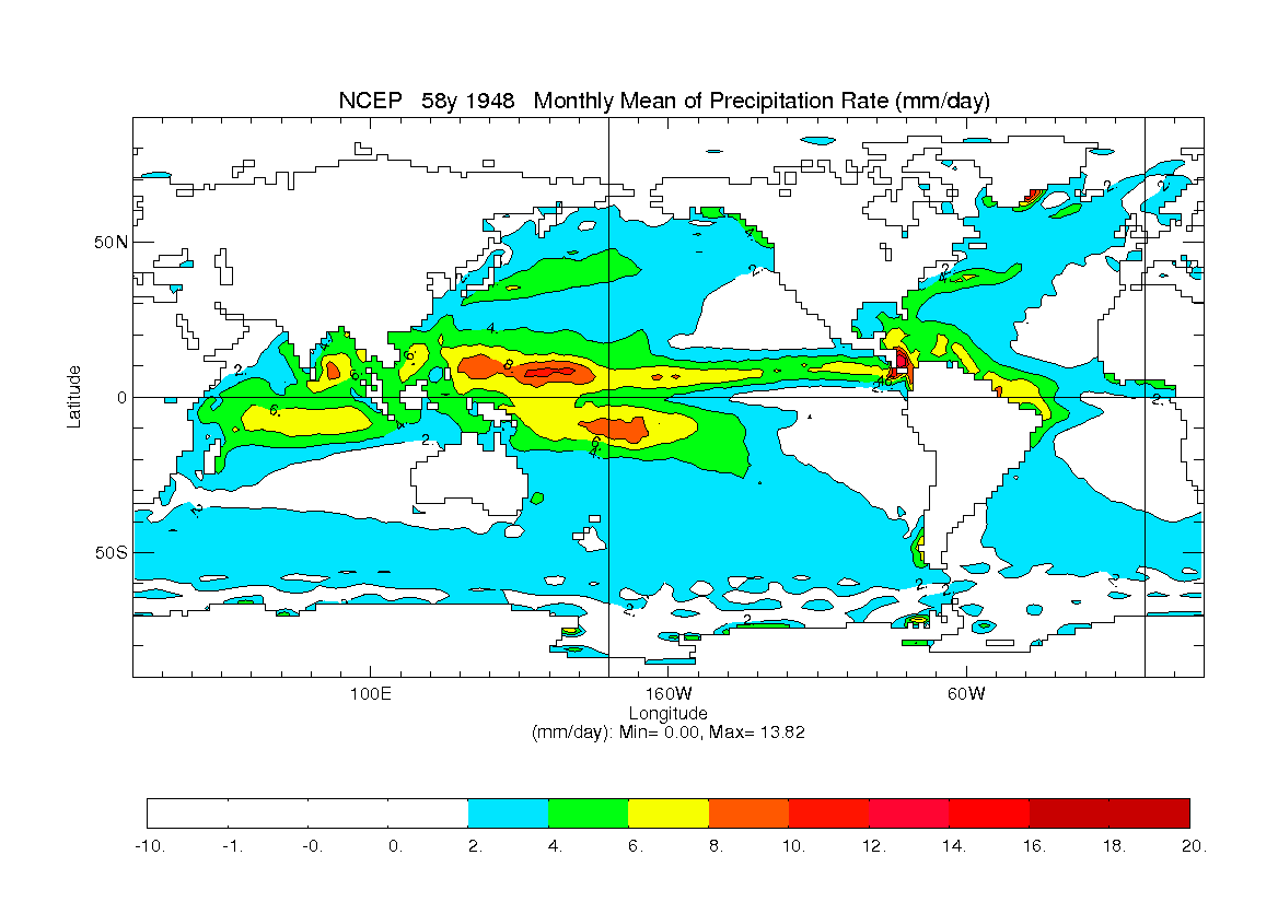
```
; grid  : grid name or @<grid> (to read grid from data file)

  'precip   1   NCEP  ncpt62  xy  58y    1948  -     1    1   v', $
```

'plt' : This parameter defines the kind of plot you want to see. It will define some features for the saxo plot routines. You can perform 2d maps, hovmoeller diagrams, simple time series, spectrum of time series...

; plt   : xy, xz, yz, x, y, z [append _<box> or _#<bathy>]
;        {xt, yt, zt, t}_<box>[@f<direc><width>][@s][@z][@r<win>]
;           <box> : defined in Default/hovmoel_box.def
;           <bathy> : first letters of bathymetry file in Default/Grids
;           <direc> : t,x,y,z = filtering/smoothing direction (default: t)
;           <width> : running mean filter width (default = 1)
;                     grid point smoothing for space
;           @r<win> : time serie stddev in running <win>dow
;           @s      : spectrum of time serie
;           @w      : wavelet of time serie
;           @z      : remove zonal mean (eddy field) from 2D field (xy
;                     plot only)
;        density bining plots : xs, ys, s [append _<box> or _#<bathy>]
;                               st_<box>[@f<direc><width>][@s]
;        statistics : @@<variable> 2D plot: plt=xyt
;

  'sosstsst    1   2L24  T     t_nino_3@s  1m@t412  186001  195912    1     1   v', $

'timeave' : The time average defines the duration on which the files have been averaged. For instance, you will have '1m', '1mm', '1y', '32y'. You may add a trend to that : do you want to remove the seasonal cycle from the time series ? Thus the trend shoud be @t412. Or if you want to write data in another netcdf file, the trend should be @t9 (in that case, you will also have to define the 'out' parameter â see below).

; timeave : <n>[m]<timeave>[@t<trend>]
;            n: integer, timeave: of d(ay),m(onth),y(ear)
;           [m] stands for mean <timeave>
;               -> requires spec for date interval (of mean):
;               [date_i]-[date_f]
;           <trend> : time serie trend type (default = 0, in this
;           case, use @t9 to
;           activate data output writing - out=data)
;           @t412: remove mean SC
;           @t41: remove mean of time serie
;

'date1' : The name of the netcdf file should have some indications of dates (for instance, 2L24_1m_186001_195912_grid_T.nc). If you only want to visualize the monthly mean SST of May 1871, you will have to specify 187105 as the 'date1' parameter. It is not compulsory to specify any final date for the 'spec' parameter in that case : '-' will be enough. The dates specified in the name of the file and the dates specified in post_it.pro should be coherent since the netcdf file only contains time steps : in our example, May, 1871 should corresponds to the 137th time step in the file. Dates can go down to daily scales (18710510) and you can even specify seconds.
```
; date1 : [yy..yyy][mm][dd]-[sssss][_<ave_period>]
;         <ave_period> for mean <timeave> : date interval <date_i>-<date_f>
;
```

'spec' : This parameter has two meanings. It may define the ending date of a 1d plot (SST anomaly averaged over nino_3 region as a function of time). But it may set parameters for a to make differences between two plots : this is the second way to make differences.
```
; spec  : time serie : date2
;         difference : d:<exp>/<timeave>/<date1>[/<spec2>]        
 
  'votemper    1   CD2   T     xz_pac_eq300  100y   1870  d:2L24/100y/1860   1     1   v', $
```

'disp' : the kind of display is set with this parameter. You can specify if you want several plots on the same window and how they will be organised on it. By default, plots are carried out with a landscape view. For the example below, 'disp' is set to '2x2' and the plot would have been the same with '2x2L'. Please notice that you don't have to set 'on' to '1' at each line : the first line is enough ; post_it understands that it has to consider four lines for the plot.
```
; disp  : multi-window display n[x<m>][<orient>]  <orient> = P  (L is default)

  'sosstsst   1    CD2  T       xy  100y   1870  d:2L24/100y/1860  2x2     1   v', $ 
  'tsol       0    CD2  lmdzl   xy  100y   1870  d:2L24/100y/1860  1     1   v', $
  'sozotaux   0    CD2  U       xy  100y   1870  d:2L24/100y/1860  1     1   v', $
  'sometauy   0    CD2  V       xy  100y   1870  d:2L24/100y/1860  1     1   v', $
```

'out' : the kind of outputs you want is set with this parameter. You may want to see 'raw' data without processing. In that case, 'out' has to be set to 'tv'. This plot will be similar to a call to 'pltv' saxo routine (you will be able to click on 2d map with your mouse and see point-to-point values). You may want to write processed data (Wind stresses standard deviations, SST anomaly averaged over nino_3 region as a function of time, ...) in another netcdf file. In that case, 'out' has to be set to 'data'. You may want to print your plot into a ps file ('ps') after having visualised it ('v') or directly print it to the printer ('psc') -> does not work ?????
```
;  out   : v (view), tv (tvnplot), ps[prt] PostScript, data (ascii,
;         requires timeave + @t9) or (t)cdf (netCDF file)
;                  prt = b : BW printer
;                  prt = c : color printer
;                  prt = t : transparent printer
;              to save postcript activate save_ps in plt_def
;              tcdf: pltt netCDF writing (t, xt, yt types)
```

Attachments (4)

2L24_HTC300_TROP_100y.gif (88.3 KB) - added by kolasinski 16 years ago.
2L24_PRECIP_OLR_XT_PACEQ_1mm_100y.gif (84.5 KB) - added by kolasinski 16 years ago.
NCEP_PRECIP_TROP_58y.gif (51.3 KB) - added by kolasinski 16 years ago.
2L24_SST-SPECTRUM_T_NINO_3_1m@t412_100y.gif (21.2 KB) - added by kolasinski 16 years ago.

Download all attachments as: .zip

Download in other formats:

Plain Text