Chap.2 : File post_it.pro

General description and a first example

post_it.pro is the file in which you will work. It defines the in line commands which will be read by post_it so as to get the plot you want. For instance :

cmdline = [ $
; var             on   exp      grid  plt   timeave  date1   spec  disp   proj   out
  'sohtc300   1     2L24   T       xy   100y      1860     -       1       1        v', $

'lastline 0' ]

This means that you want the sohtc300 variable to be visualised from a netcdf file called '2L24_100y_1860_*_grid_T.nc' on a 2D plot 'xy'.
The result is the following picture (the quality is better in "ps" format than in "gif" format below).

As a consequence, the names of the netcdf files are standardized and follow this pattern :
'Experiment'_'Frequency'_'Date1'_'Date2'_'Grid Type'.nc

More details about the variables defined in 'post_it.pro'

• Variable 'spec_base_list' defines where to find a specific database of files. It should begins with the name of the experiment (here all files beginning with 'CMAP_')

  spec_base_list = [ $ 
   'CMAP = local:/home2/mkdlod/database/CORREL/', $
  ' ']
  

• Variable 'data_base_list' defines also where to find by default all the databases ('ncdf_db'). Il also allows to define generic databases. For instance, 'MRI_db' defines all files beginning with 'MRI' : it can be 'MRI_', 'MRIoCTL', 'MRIo2X'...

  data_base_list =  [ $
  'ncdf_db = local:/home2/mkdlod/database/', $
  'MRI_db = local:/home2/mkdlod/ERIC-LSCE/database/IPCC/',  $
  ' ']
  

• Variable 'out_ps' defines where to find the postscripts files generated and puts them in the 'iodir' directory.

  out_ps = homedir+'/Post_out/'
  

• Variables 'prt_BW', 'prt_col', 'prt_tra' define the unix print command you want to use for printing postscripts files. This does not work at the moment in my case !!!!!!

  prt_BW  = 'lpl'
  prt_col = 'x4'
  prt_tra = 'lprdgt'
  

• Variable 'lp_opt'

  lp_opt = ''
  

• Variable 'ghost'

  ghost = 'lpg'
  

• Variable 'out_all' : if you want to override all the local 'out' options (each in line command has a specific 'out' option). For instance, you visualised 10 plots already and you want to print them all. Instead of setting all the individual in line 'out' options, you set 'out_all' to 'ps' once and for all. By default, it shoud be set to '-' to avoid to override local 'out' options.

  out_all = '-'
  

• Variable 'other_file' : Instead of using the file 'post_it.pro' to read the in line commands, you would like to use another file ('post_it.pro' might be too big).

For this purpose, set the variable 'other_file' to the name of the other file. By default, it is set to '-', which means 'post_it.pro' has to be read. Pay attention to the fact that the structure of the other file is bit different from 'post_it.pro' since you should only find the 'cmdline2' variable (similar to 'cmdline' from 'post_it.pro') in it.

other_file = 'post_it2'
other_file = '-'

• Variable 'cmdline' : In this very long variable, you set the plot you want to see or print. Please check the other example below :

  cmdline = [ $
  ; var        on   exp     grid  plt               timave   date1                spec                    disp   proj   out
    'precip   1   2L24  lmdzl  xt_pac_eq  1mm     01_1860-1959  12_1860-1959     2P     1        v', $
    'topl     0   2L24  lmdzl  xt_pac_eq  1mm     01_1860-1959  12_1860-1959     1       1        v', $
  
  'lastline 0' ]
  

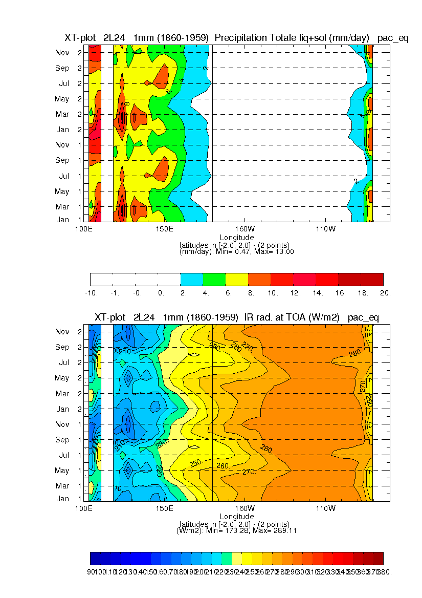
This in line command allows to see 2 plots on the same window ('Paysage' format). These are the seasonnal cycle of precipitation (called precip) and OLR (called topl) for the '2L24' experiment along the equator ('x' -> longitude, 't' -> time). The variable is averaged zonally on the box 'pac_eq' which is defined in 'domain_boxes.def' file. The grid type is 'lmdzl'. The file should contains 12 mean months from January to December and those mean months are carried out on 100 years from 1860 to 1959. The result is the following picture.