| Revision History | |
|---|---|
| Revision 0.0 | May 29, 2000 |
| French release by Sébastien Masson | |
| Revision 0.1 | July, 2002 |
| Translation by Albert Fisher | |
| Revision 0.2 | July 20, 2006 |
| HTML to XML/Docbook migration by Françoise Pinsard | |
| Revision 1.0 | August, 2006 |
| Major update by Steve Navarro | |
| Revision 1.1 | September, 2006 |
| Review by Sébastien Masson | |
| Revision 1.2 | April 2008 |
| migration from DocBook 4.2 to Docbook 5.0 | |
Table of Contents
There is several ways to launch XXX which we will detail in the next sections:
    idl> xxx
    idl> xxx, /separate
    idl> xxx, restore = 'file.dat'
    idl> xxx, 'file.nc'
    idl> xxx, 'file.nc', keywd1 = …, keywd2 = …
    idl> xxx, 'file.nc', 'initgrid'
    idl> xxx, 'file.nc', 'initgrid', keywd1 = …, keywd2 = …
    idl> xxx, 'file.nc', 'initgrid', 'arg1, arg2, …'
A window will open with 3 parts to consider.
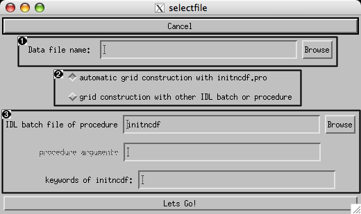


The name of the data file. It can be typed directly in the window provided, or selected with the help of the button.
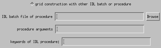
For visualising grilled data, you need to define the grid on which are located the data. By default, is checked. This means that the grid will be defined by using the informations contained in the data file (through the IDL prodecure initncdf) without needing any other auxiliary file. If you checked , this means that you don't want to use the default initncdf procedure to define the grid and you will provide your own IDL procedure or the so-called IDL batch file (a file which is called by using @, see IDL documentation).
This third part allows you to specify the name, the argument and the keywords of the routine you want to use to initialize the grid. By default the name of the procedure is initncdf, its argument will be automatically defined so you cannot change them. If you checked , you have to select the name of the IDL procedure or batch file and its suitable arguments and keywords. Note that if you select an IDL batch file you cannot give any parameter or keyword.
Once these two lines have been completed, click on .
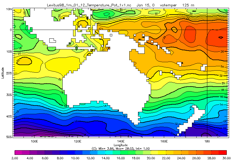
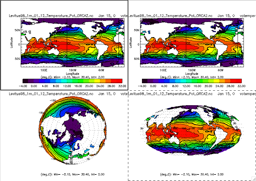
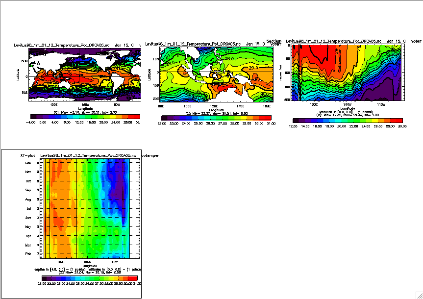
For example, we choose the IDL batch file tst_initlev. Compare the result with checked. Cf Figure 18, “temperature of the ocean at depth 125 meters without proper land/sea mask”
This is the same as the simple Section 1.1, “idl> xxx” except that once the xxx window open, you will have 2 separate windows (command and plotting window) instead of one.
In that case xxx window will open directly in the same state as it was when the file file.dat was created. see ???.
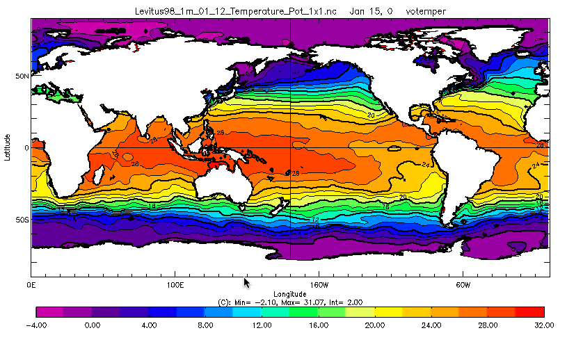
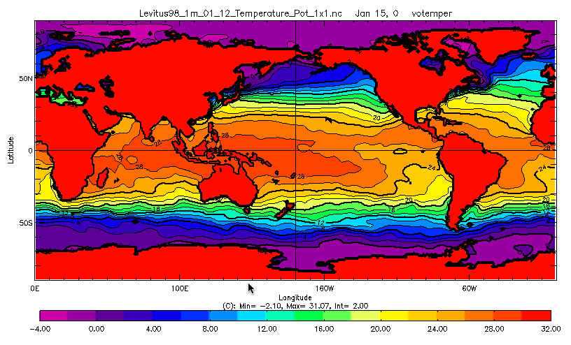
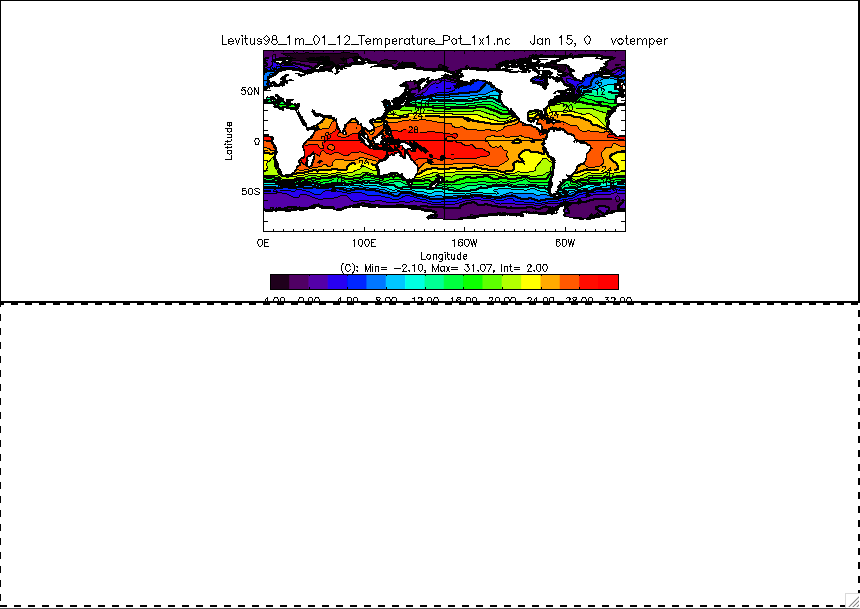
In this case, the xxx window directly open the data file file.nc and build the grid automatically with the IDL procedure initncdf. For example:
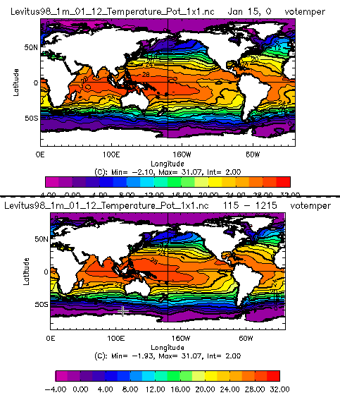
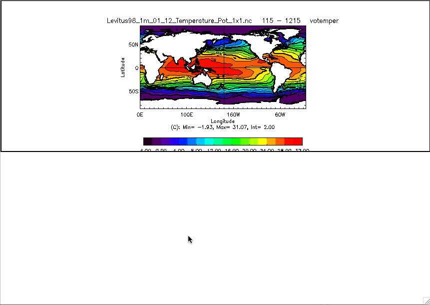
idl> xxx, 'Levitus98_1m_01_12_Temperature_Pot_1x1.nc'
In this case, the xxx window directly open the data file file.nc, build the grid automatically with the IDL procedure initncdf and use the keywords keywd1 = …, keywd2 = …
idl> xxx, 'Levitus98_1m_01_12_Temperature_Pot_1x1.nc', useasmask = 'votemper', missing_value = 31.0720
In this case, the xxx window directly open the data file file.nc and build the grid directly with the IDL procedure or batch file initgrid
idl> xxx, 'Levitus98_1m_01_12_Temperature_Pot_ORCA2.nc', 'tst_initorca2'
In this case, the xxx window directly open the data file file.nc, build the grid directly with the IDL procedure initgrid and use the keywords keywd1 = …, keywd2 = …
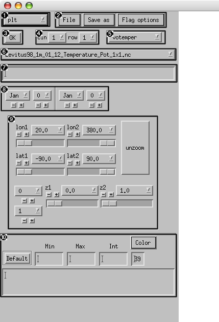
Figure 4. Window xxx 2
|
Plot type |
|
Menu |
|
OK |
|
Page layout |
|
Variables list |
|
Files list |
|
Command text |
|
Calendar |
|
Domdef |
|
Spefications |


Allows specification of the type of plot desired.
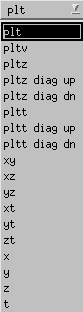
Note
If the type plt is selected, the selection of plot type
is made by mouse. Cf Section 3.1, “In the graphics window on a horizontal plot”
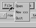
to open a new file. Same procedure as during the Section 1.1, “idl> xxx”. The new file can be on a different grid, with different variables, with a different time base …
to open a second XXX window identical to the first one.
to close the XXX window.
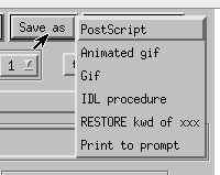
to save the plotting window in Postscript format
to create an animation of the plotting window.
Note
The creation of an animation is only possible if none of the plots have a time axis, and if the plots are all on the same time base (calendar). On the other hand, animations of horizontal and vertical plots, with different color palettes (for those not on an X-terminal), are possible.
Note
The creation of animations has a tendency to saturate the video memory of X-terminals, crashing the entire program …
to save a gif of the plotting window.
to save the command history that has created the plot in an IDL procedure that can be re-executed later. For example if I save the commands in
xxx_figure.profile, when ever I want, I can then launch a new IDL session and type:idl>@initidl>xxx_figureand I'll obtain the saved figure.
idl>xxx_figure,/postor
idl>@pswill then create a Postscript file of the figure.
-
to save the xxx widget (all buttons and parameters stored in memory …) in a binary file in order to quit xxx and relaunch it later like in Section 1.3, “idl> xxx, restore = 'file.dat'” and get exactly the same configuration.
-
lists in the IDL window the command history that created the last plot. Useful primarily for debugging…
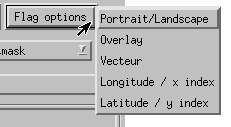
changes the configuration of the plot.
to plot contours of a different field on top the one represented as color-filled contours. It is necessary to relaunch the entire plot to make this work!
to plot a vector field on top of contours. Only works on horizontal plots (
plt.pro). As for Overlay, a relaunch of the entire plot is necessary.switches longitude labeling of the plot sub-domain from degrees to indexes following i.
switches latitude labeling of the plot sub-domain from degrees to indexes following j.
Caution
Careful, a selected option remains selected until it is re-clicked.
Specify the number of columns and rows for plots on the sheet of paper.
You can choose the variable to work on.

You can choose the file to work on.
To specify in the widget part number 7 the computation you want to do on the data
Note
In all cases bellow, the name given to a field (a, b, c, …) is of no importance.
If you want to make basic linear computation (like difference between fields, add/multiply by a constant …), you can simply put the following commands: a - bnumb1*aa + numb or any command with the following format numb1*a + numb2*b + numb3*c … + numb where numb1, numb2, … correspond to numbers and a, b, c … will be the data to read.
The calendar is made up of two drop-lists, which allow specification of two dates, the beginning and end of a time series, or the period over which to average before plotting.
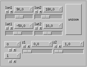
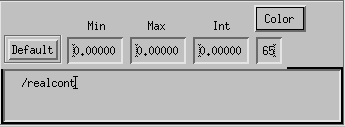
A series of widgets that allow specification of the min/max limits of the domain in longitude/x-index, latitude/y-index, and depth in levels or meters.
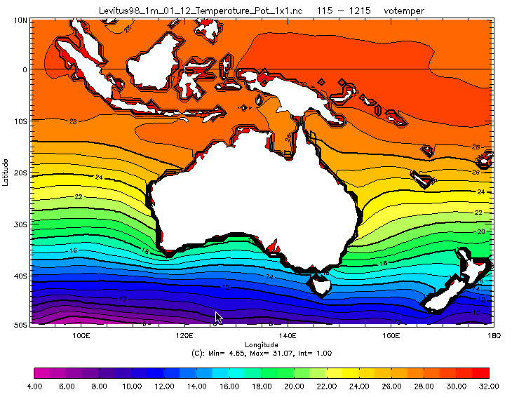
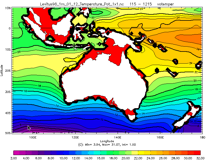
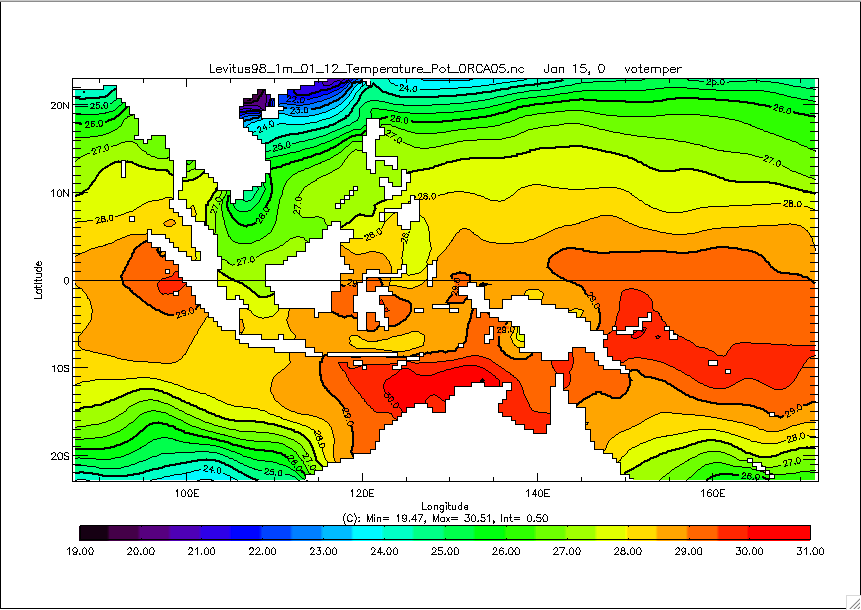
As you can see, at this depth, we better define a land/sea mask when loading the grid. Cf Figure 3, “Oceania at 125 meters of depth with proper grid initialization”
You can restore configuration by default by pressing the button.
Note
The path of the file definedefaultextra.pro that defines the default values for each variable names is displayed when the cursor hovers over the button . This file contains a case statement based on the name of the variable and defining the min, max, contour interval and other keywords that should be used as default for the specified variable. You can copy this file in your own ${HOME}/My_IDL/ directory and easily modify it to suit your favorite default values.
For the color palette, you can either specify the name or go search for one among the palettes available.
The “keywords” window allows specification of all desired keywords. There is a few examples of the use of this “keywords” window.
![Add /realcont, map=[90,0,0], /ortho, cell_fill=2 keywords](figpng/xxx_0211a.png)
![Graphic with /realcont, map=[90,0,0], /ortho, cell_fill=2 keywords](figpng/xxx_0211.png)
Select a domain and select the horizontal plot (plt), vertical plot
(pltz), or the hovmoeller plot (pltt):
The domain we'd like to select for the plot is determined by one of its diagonals, defined therefore by two points. The first point is defined when the mouse button is pushed, then the mouse is moved, and the second point is defined as the mouse button is released (click-drag). The domains are thus defined by a long click (LC). To determine which type of plot should be made of selection, use:
If the plot selector is on plt
the mouse button to create horizontal plots (
plt)the mouse button to create vertical plots (
pltz)the mouse button to create common hovmoellers for xt and yt cuts (
pltt)
In summary:


Note
If the plot selector is on something other than plt the indicated plot type is made.
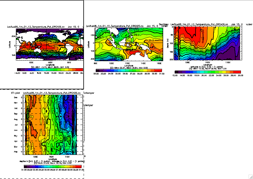
Select the number of columns and rows for the page.
Create a first plot. It will appear in the first frame.
To create a plot in another frame double-click in the frame with the button (). A black dotted frame will surround the designated frame, the “target” frame. A black frame will surround the first plot. This is the “reference” frame, in other words the one that all the XXX widgets refer to. Change for example the date and create a new plot. With a button double-click in the first frame, all the widgets change and refer again to the first plot. A double-click with the button in the second frame will erase the plot.
In summary:


Here's a series of commands to show how this works.
-
Load xxx with the command:
idl>xxx,'Levitus98_1m_01_12_Temperature_Pot_ORCA05.nc','tst_initorca05' -
Select a 3-D field and create 6 frames for the sheet of paper.
-
Create a horizontal plot in Frame 1
-
DCM in frame 2, LCL on the plot in frame 1 to create a horizontal zoom in frame 2.
DCM in frame 3, LCM on the plot in frame 1 to create a vertical cut in frame 3.
DCM in frame 4, LCR on the plot in frame 1 to create a hovmoeller in frame 4.
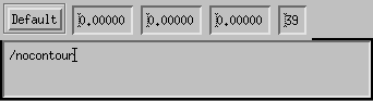
To redo the hovmoeller with the keyword
/nocontour
-
DCL in frame 4 which now becomes the reference and target frame.
-
Add the keyword
/nocontour
-
Click , and the plot is redone.
-
In the IDL window type (as many time you click on a button since a problem occurs in xxx !!!),
idl>retall -
In the IDL window, type
idl>domdef -
DCR to erase the problem frame.
-
change the orientation of the plot by pressing → . Cf Section 2.2.3, “Flag options sub-menu”
-
quit XXX cleanly using from the menu. Cf Section 2.2.1, “File sub-menu”
Note
Always avoid if at all possible closing and killing the XXX window, but rather select from the menu. XXX uses a large number of pointers, and want only killing the window will leave a large number of unused variables in memory, which could in the end overflow. To clean up this memory:
idl>ptr_free, ptr_valid()