| Revision History | |
|---|---|
| Revision 0.0 | 29 July 2005 |
| First draft | |
| Revision 0.1 | 29 August 2005 |
| last Japanese version! | |
| Revision 0.2 | May 2006 |
| split with getsaxo | |
Table of Contents
In this document, we supposed that you followed Get SAXO recommandations.
Each IDL session using SAXO
must always start with: idl>
@init.
The @ is equivalent to an include. It is used to execute a set of IDL commands that will be directly executed without any compilation (as it is the case for a procedure or a function). All variables defined and used in the @... file will still be accessible after the execution of the @... is finished (which is not the case for procedures and functions that ends with the return instruction).
$cd${HOME}/My_IDL/$idlIDL Version 6.0, Mac OS X (darwin ppc m32). (c) 2003, Research Systems, Inc.Installation number: 35411.Licensed for personal use by Jean-Philippe BOULANGER only.All other use is strictly prohibited.idl>@init% Compiled module: KEEP_COMPATIBILITY.% Compiled module: FIND.% Compiled module: PATH_SEP.% Compiled module: STRSPLIT.% Compiled module: DEF_MYUNIQUETMPDIR.We forget the compatibility with the old version% Compiled module: DEMOMODE_COMPATIBILITY.% Compiled module: ISADIRECTORY.% Compiled module: LCT.% Compiled module: RSTRPOS.% Compiled module: REVERSE.% Compiled module: STR_SEP.% Compiled module: LOADCT.idl>
As an IDL session using SAXO
must always start with idl>
@init, it could be
convenient to define the environment variable IDL_STARTUP to ${HOME}/My_IDL/init.proinit.pro will automatically been
executed when starting IDL. This can be done with the following
command:
- csh
-
$setenvIDL_STARTUP${HOME}/My_IDL/init.pro - ksh
-
$exportIDL_STARTUP=${HOME}/My_IDL/init.pro
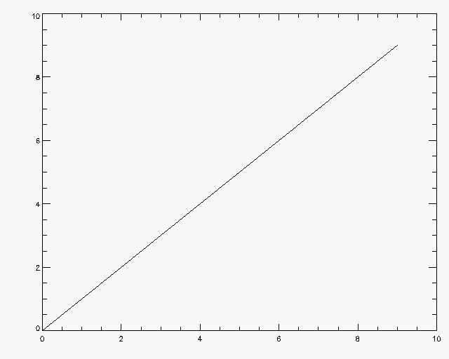
idl>n = 10
idl>y = findgen(n)idl>plot, y
|
findgen stands for float index generator.
|
Using IDL plot
command is quite inconvenient to save the figure as a postscript.
In addition, positioning the figure on the window/page by using
!p.position, !p.region and !p.multi is often a nightmare. That's why we
developed splot (like
super-plot) which can be used in the same way as plot but is much
more convenient to make postscript and position the figure.
idl>splot, y% Compiled module: SPLOT.% Compiled module: REINITPLT.% Compiled module: PLACEDESSIN.% Compiled module: CALIBRE.% Compiled module: GIVEWINDOWSIZE.% Compiled module: GET_SCREEN_SIZE.% Compiled module: TERMINEDESSIN.
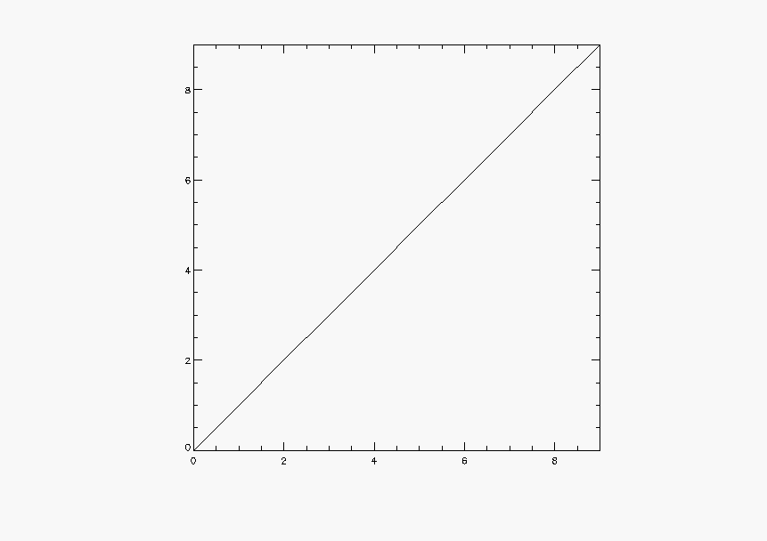
Save the figure seen on the screen as a (real, not a screen capture) postscript in only one command.
idl>@ps% Compiled module: GETFILE.% Compiled module: PUTFILE.% Compiled module: OPENPS.% Compiled module: XQUESTION.Name of the postscript file? (default answer is idl.ps)first_ps% Compiled module: ISAFILE.% Compiled module: XNOTICE.% Compiled module: CLOSEPS.% Compiled module: PRINTPS.% Compiled module: FILE_WHICH.% Compiled module: CW_BGROUP.% Compiled module: XMANAGER.
|
If needed, the name of the postscript
will automatically be completed with .ps. Just hit return, if you
want to use the default postscript name: |
Check that the “first_ps.ps” file is now
existing...
idl>print, file_test(psdir + 'first_ps.ps')1idl>help, file_info(psdir + 'first_ps.ps'), /structure** Structure FILE_INFO, 21 tags, length=64, data length=63:NAME STRING '/Users/sebastie/IDL/first_ps.ps'EXISTS BYTE 1READ BYTE 1WRITE BYTE 1EXECUTE BYTE 0REGULAR BYTE 1DIRECTORY BYTE 0BLOCK_SPECIAL BYTE 0CHARACTER_SPECIALBYTE 0NAMED_PIPE BYTE 0SETUID BYTE 0SETGID BYTE 0SOCKET BYTE 0STICKY_BIT BYTE 0SYMLINK BYTE 0DANGLING_SYMLINKBYTE 0MODE LONG 420ATIME LONG64 1122424373CTIME LONG64 1122424373MTIME LONG64 1122424373SIZE LONG64 4913
splot accepts the
same keywords as plot
(/ISOTROPIC, MAX_VALUE=value, MIN_VALUE=value,
NSUM=value, /POLAR, THICK=value, /XLOG, /YLOG, /YNOZERO),
including the graphics keywords (BACKGROUND,
CHARSIZE, CHARTHICK, CLIP, COLOR, DATA, DEVICE, FONT, LINESTYLE,
NOCLIP, NODATA, NOERASE, NORMAL, POSITION, PSYM, SUBTITLE, SYMSIZE,
T3D, THICK, TICKLEN, TITLE, [XYZ]CHARSIZE, [XYZ]GRIDSTYLE,
[XYZ]MARGIN, [XYZ]MINOR, [XYZ]RANGE, [XYZ]STYLE, [XYZ]THICK,
[XYZ]TICKFORMAT, [XYZ]TICKINTERVAL, [XYZ]TICKLAYOUT, [XYZ]TICKLEN,
[XYZ]TICKNAME, [XYZ]TICKS, [XYZ]TICKUNITS, [XYZ]TICKV,
[XYZ]TICK_GET, [XYZ]TITLE, ZVALUE).
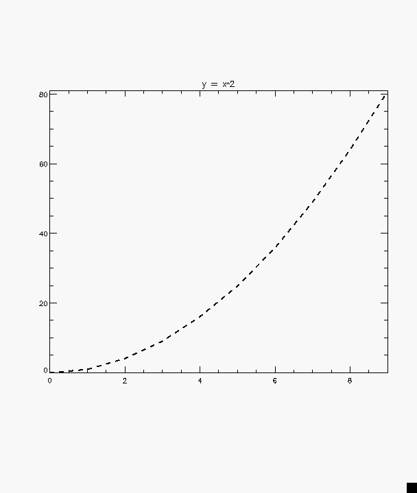
It can therefore be customized as much as you want. See this short example:
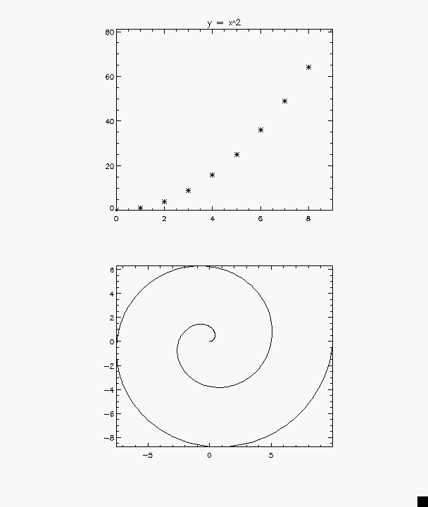
idl>splot, y, y^2, linestyle = 2, thick = 2, title = 'y = x^2', /portrait
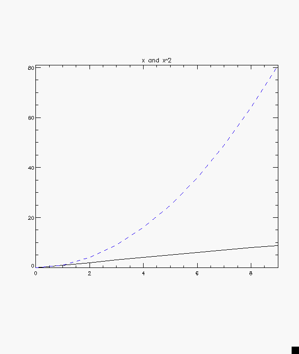
splot can be used
to setup the graphic environment (!p,
!x, !y,
!z variables) needed by procedures
like oplot
idl>splot, y, yrange = [0, (n-1)^2], title = 'x and x^2'idl>oplot, y^2, color = 50, linestyle = 2
Use the keyword small to produce multi plots figures.
  idl> splot, y, y^2, title = 'y = x^2', psym = 2, small  = [1, 2, 1]
  idl> splot, findgen(360)/36., findgen(360)*2.*!dtor, /polar $
  idl>     , small  = [1, 2, 2], /noerase
|
the |
|
you must put /noerase otherwise the second plot will be
done in a new window. |
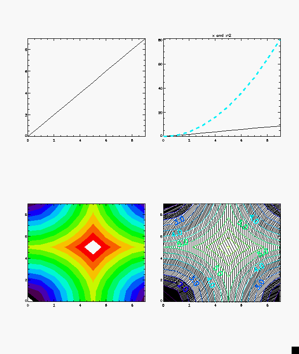
Following splot example, we provide scontour as a "super contour".
idl>z = dist(n)% Compiled module: DIST.idl>scontour, z% Compiled module: SCONTOUR.% Compiled module: CHKSTRU.
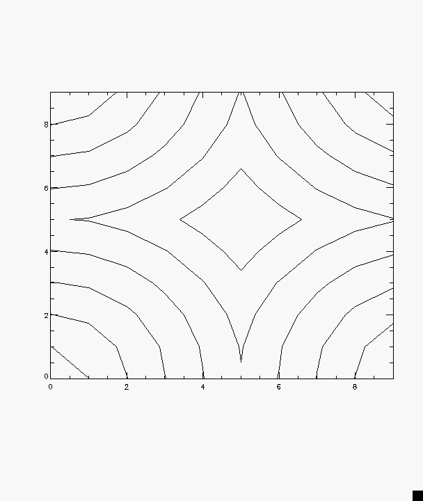
scontour accepts
the same keywords as contour (C_ANNOTATION=vector_of_strings, C_CHARSIZE=value,
C_CHARTHICK=integer, C_COLORS=vector, C_LABELS=vector{each element
0 or 1}, C_LINESTYLE=vector, { /FILL | /CELL_FILL |
C_ORIENTATION=degrees}, C_SPACING=value, C_THICK=vector, /CLOSED,
/DOWNHILL, /FOLLOW, /IRREGULAR, /ISOTROPIC, LEVELS=vector,
NLEVELS=integer{1 to 60}, MAX_VALUE=value, MIN_VALUE=value,
/OVERPLOT, {/PATH_DATA_COORDS, PATH_FILENAME=string,
PATH_INFO=variable, PATH_XY=variable}, TRIANGULATION=variable,
/PATH_DOUBLE, /XLOG, /YLOG, ZAXIS={0 | 1 | 2 | 3 | 4}),
including the graphics keywords (except
LINESTYLE, PSYM, SYMSIZE).
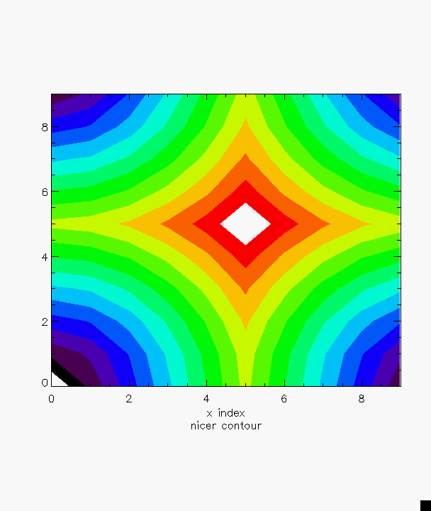
It can therefore be customized as much as you want. See these short examples:
idl>scontour, z, /fill, nlevels = 15, subtitle = 'nicer contour' $idl>, xtitle = 'x index', charsize = 1.5
It can be used in combinaison with contour to make more complex plots:
  idl> ind = findgen(2*n)/(2.*n)
  idl> scontour, z, levels = n*ind, c_orientation = 180*ind, c_spacing = 0.4*ind
  idl> contour, z, /overplot, c_label = rebin([1, 0], 2, n) , levels = n*ind $
  idl>     , c_charthick = 2, c_charsize = 1.5, c_colors = 250*ind
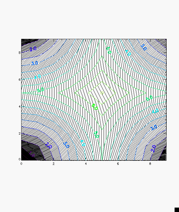
|
rebin is used to build an array containing an alternation of 1 and 0 in order to label one contour every two contours.
|
scontour is
compatible with the positioning method associated with the
small keyword. See for example
the test file tst_basic.pro:
idl>tst_basic
tvplus is a enhanced version of tvscl and allow you to have a quick look and perform basic exploration of 2D arrays.
            idl> tvplus, dist(20)
  left button  : mouse position and associated array value
  middle button: use it twice to define a zoom box
  right button : quit
  (x, y) = (  5,   5), value = 7.07107
  (x, y) = ( 12,   8), value = 11.3137
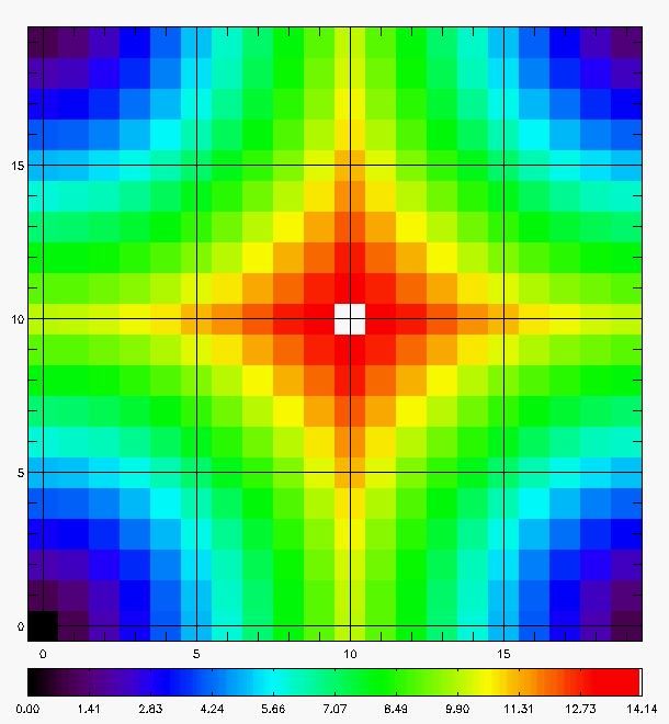
For more informations on tvplus, try:
idl>xhelp, 'tvplus'
This section briefly describes the main functionalities offered by SAXO to explore gridded data on regular or irregular grid.
As we focus in this section on the gridded data, we must first
load the grid informations before reading and plotting the data.
Loading the grid independently of the data allow you to reload the
grid only when it is strictly necessary and not every time you
access the data. In ${HOME}/SAXO_DIR/Tests/
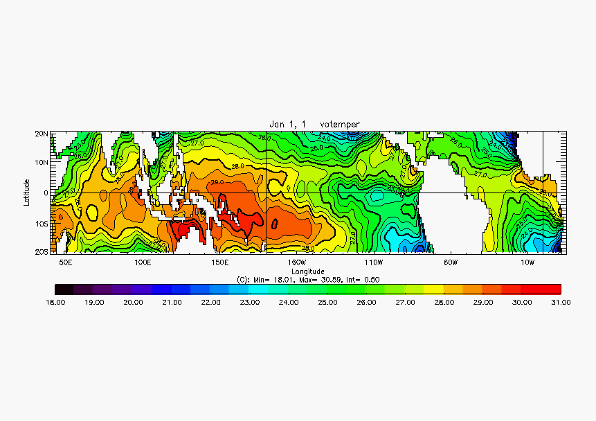
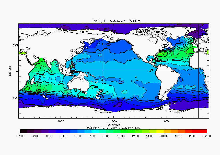
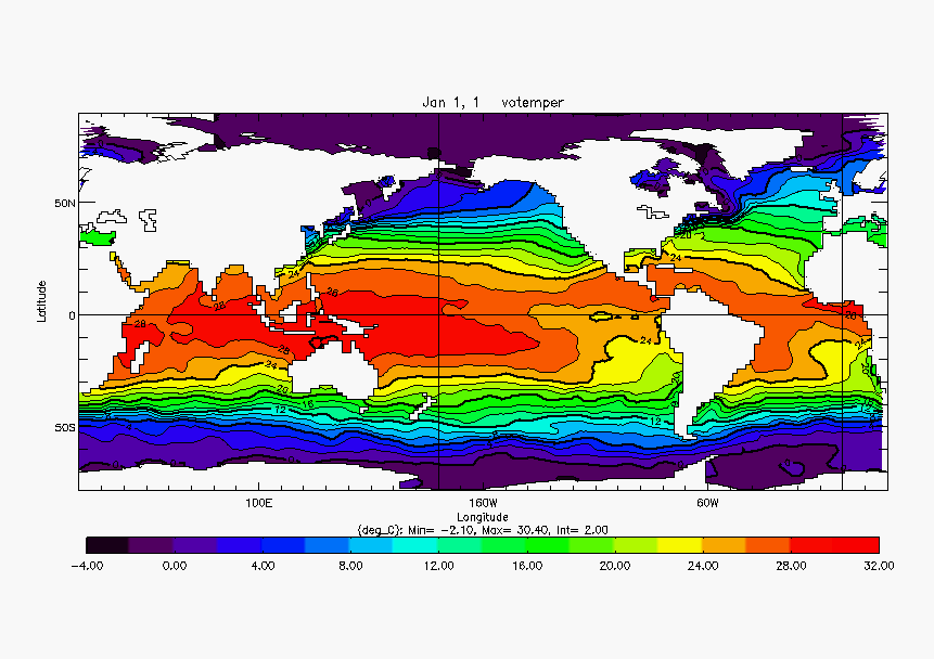
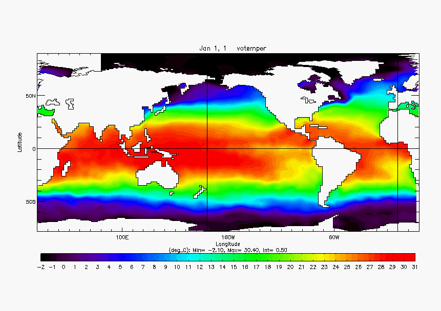
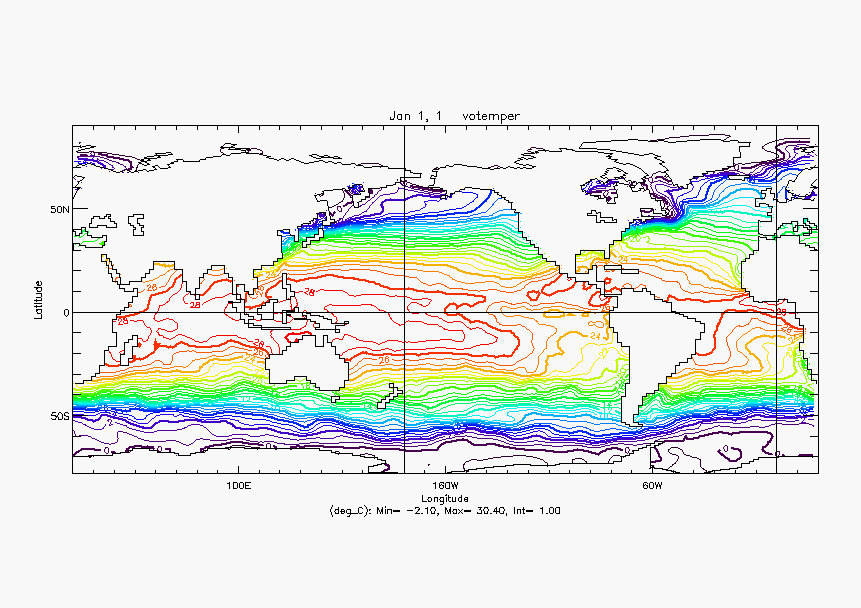
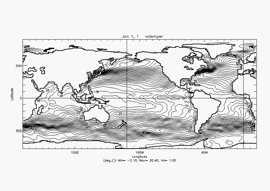
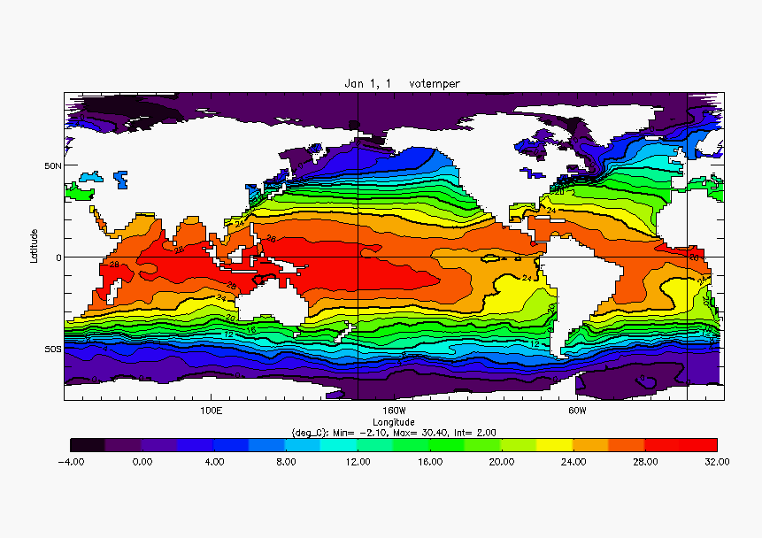
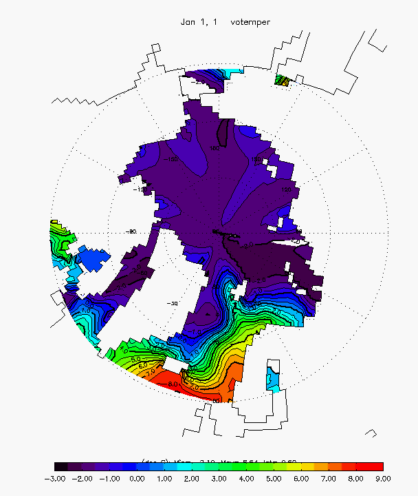
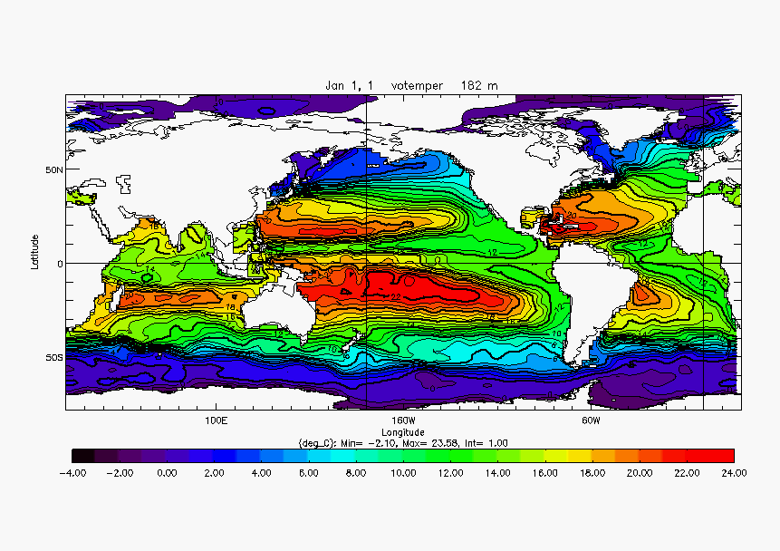
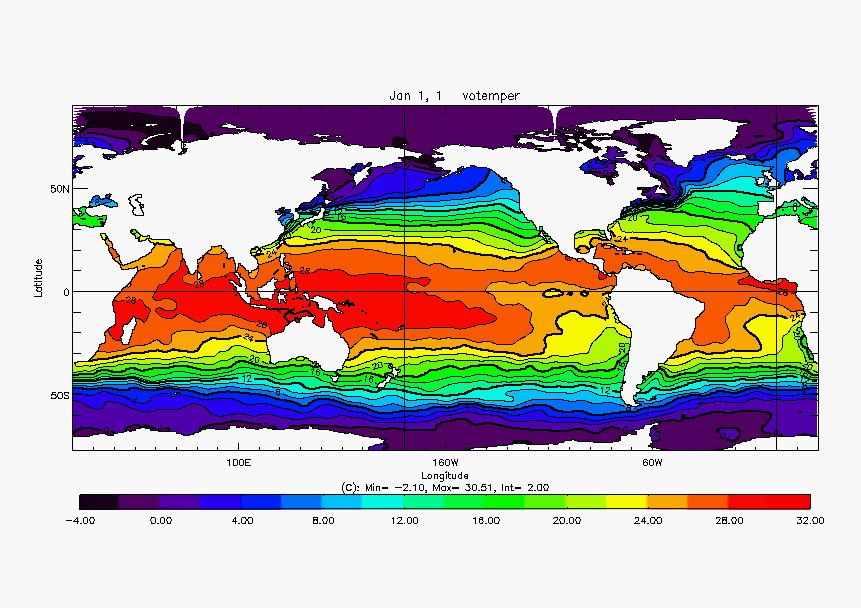
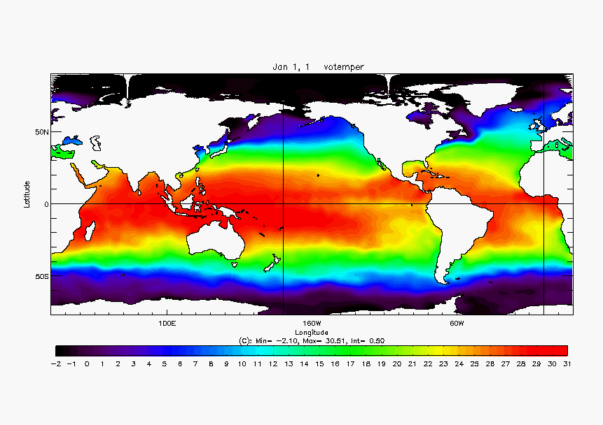
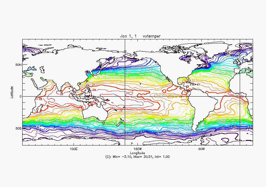
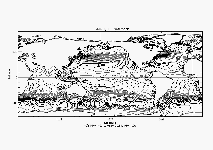
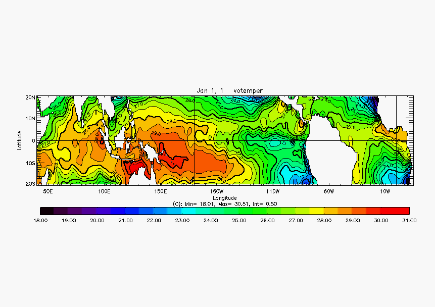
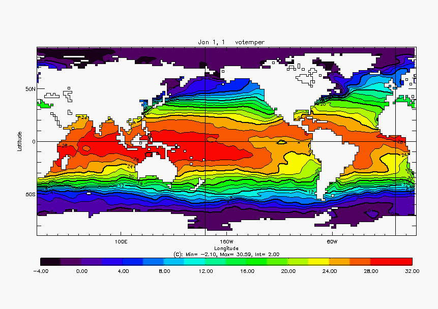
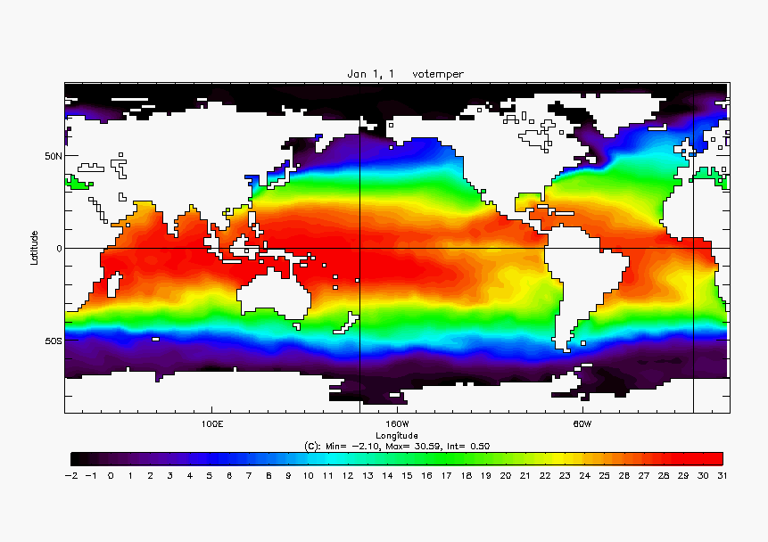
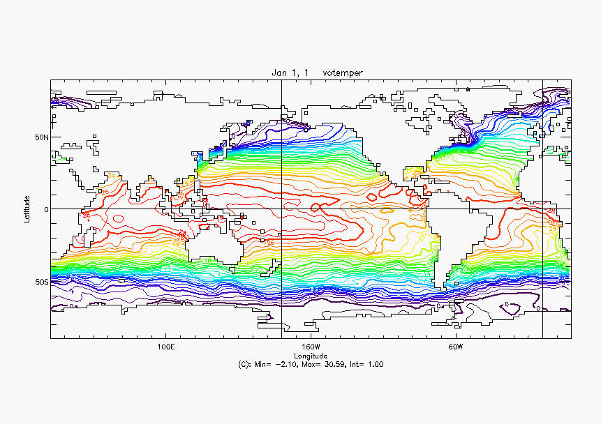
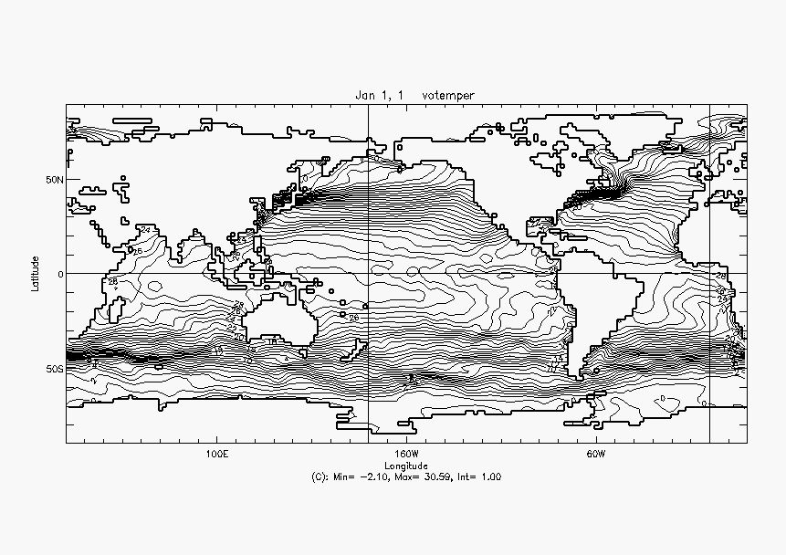
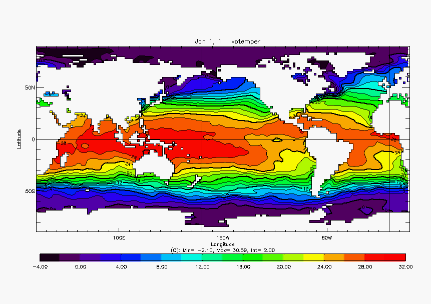
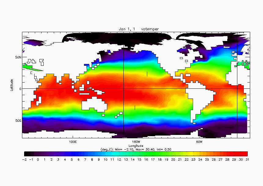
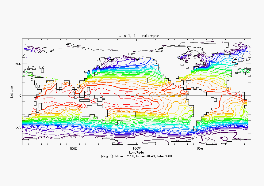
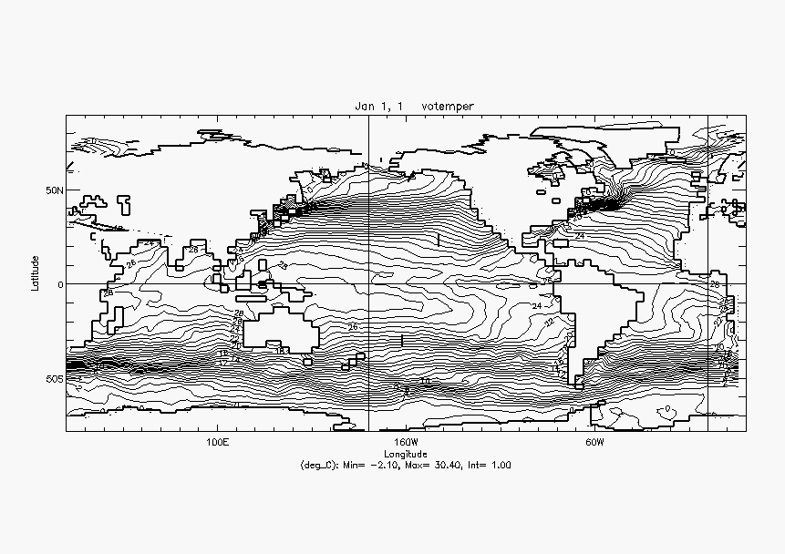
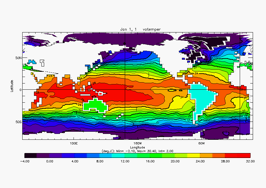
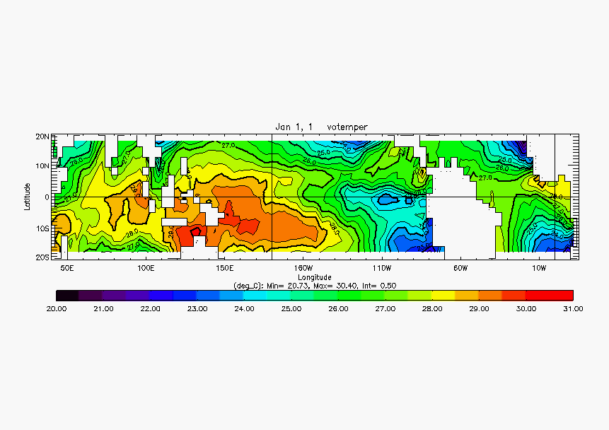
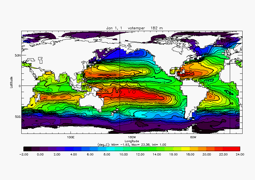
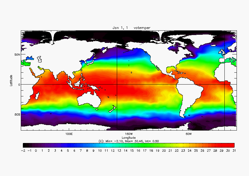
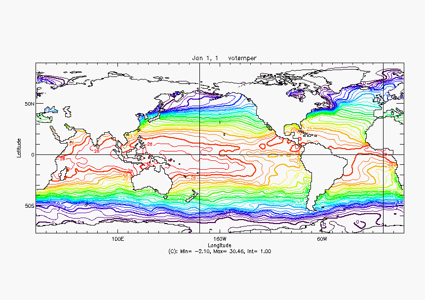
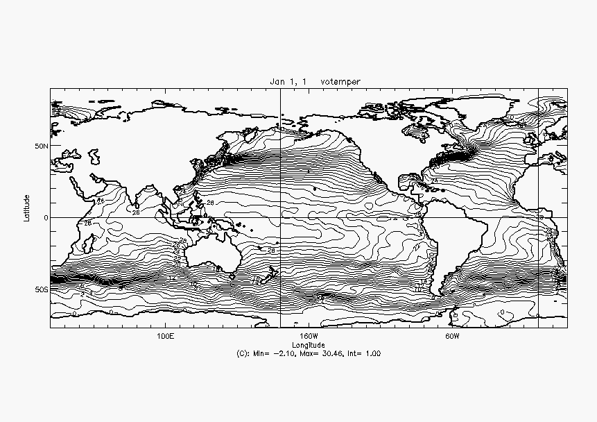
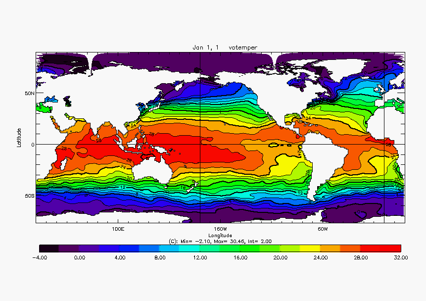
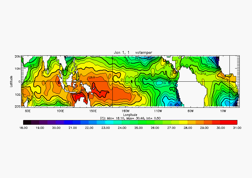
Example of Levitus temperature on a regular 1x1 grid.
idl>@tst_initlev% Compiled module: INITNCDF.% Compiled module: ISAFILE.% Compiled module: UNIQ.% Loaded DLM: NCDF.% Compiled module: COMPUTEGRID.% Compiled module: DOMDEF.% Compiled module: INTER.% Compiled module: TRIANGULE.% Compiled module: TRIANGULE_C.% Compiled module: UNDEFINE.% Compiled module: TESTVAR.% Compiled module: DIFFERENT.% Compiled module: DEFINETRI.
This @tst_initlev command allows us to define:
- domain dimensions, stored in
jpi, jpj and jpk - points abscissa, stored in 2D array glamt
- points ordinates, stored in 2D array gphit
- points depths, stored in 1D array gdept
- cells corners abscissa, stored in 2D array glamf
- cells corners ordinates, stored in 2D array gphif
- cells upper boundary depth, stored in 1D array gdepw
- land-sea mask, stored in tmask
- the cells size in the longitudinal direction, stored in 2D array e1t
- the cells size in the latitudinal direction, stored in 2D array e2t
- the cells size in the vertical direction, stored in 1D array e3t
- the triangulation used to fill the land points, stored in triangles_list
idl>help, jpi,jpj,jpkJPI (LOCAL_COORD) LONG = 360JPJ (LOCAL_COORD) LONG = 180JPK (LOCAL_COORD) LONG = 33idl>help, glamt, gphit,glamf, gphifGLAMT (LONGITUDES) FLOAT = Array[360, 180]GPHIT (LATITUDES) FLOAT = Array[360, 180]GLAMF (LONGITUDES) FLOAT = Array[360, 180]GPHIF (LATITUDES) FLOAT = Array[360, 180]idl>help, gdept, gdepwGDEPT (VERTICAL) FLOAT = Array[33]GDEPW (VERTICAL) FLOAT = Array[33]idl>help, e1t, e2t, e3tE1T (SCALE_FACTORS) FLOAT = Array[360, 180]E2T (SCALE_FACTORS) FLOAT = Array[360, 180]E3T (VERTICAL) FLOAT = Array[33]idl>help, tmaskTMASK (MASKS) BYTE = Array[360, 180, 33]idl>help, triangles_listTRIANGLES_LIST (LIEES_A_TRIANGULE) LONG = Array[3, 128880]idl>tvplus, glamt*tmask[*,*,0]idl>tvplus, gphit*tmask[*,*,0]
We provide other initialization methods/examples
- @tst_initorca2_short : ORCA2 example
- @tst_initorca05_short : ORCA05 example
- @tst_initlev_stride : same as @tst_initlev but we skip on point over 2 in x and y direction
- @tst_initorca2_short_stride : ORCA2 with stride
- @tst_initorca05_short_stride : ORCA05 with stride
- @tst_initlev_index : in that case we load the grid using points index as axis instead of the longitude/latitude position
- @tst_initorca2_index : load ORCA2 as it see by the model
- @tst_initorca05_index : load ORCA05 as it see by the model
- @tst_initlev_index_stride : @tst_initlev_index with stride
- @tst_initorca2_index_stride : ORCA2 in index with stride
- @tst_initorca05_index_stride : ORCA05 in index with stride
When the grid is really irregular (its abscissa and ordinate
cannot be descried by a vector), loading the grid directly from the
data forces us to make an approximation when computing the grid
corners position and the cells size. In that case, it can be
preferable to load the grid from the meshmask file created by OPA.
As OPA use a Arakawa-C discretization, loading the grid from the
meshmask will also define all parameters related to the U, V and F
grids (glam[uv],gphi[uv], e[12][uvf]). Note that, when using a
simple
grid definition from the data itself (with initncdf or computegrid), adding the keyword /FULLCGRID leads
also to the definition of all U, V and F grids parameters. There is
the examples to load ORCA grids from OPA meshmask.
- @tst_initorca2 : ORCA2
- @tst_initorca05 : ORCA05
- @tst_initorca2_stride : ORCA2 with stride
- @tst_initorca05_stride : ORCA05 with stride
- @tst_initorca2_index : load ORCA2 as it see by the model
- @tst_initorca05_index : load ORCA05 as it see by the model
- @tst_initorca2_index_stride : ORCA2 in index with stride
- @tst_initorca05_index_stride : ORCA05 in index with stride
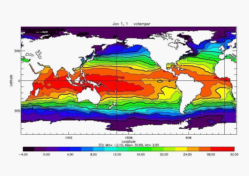
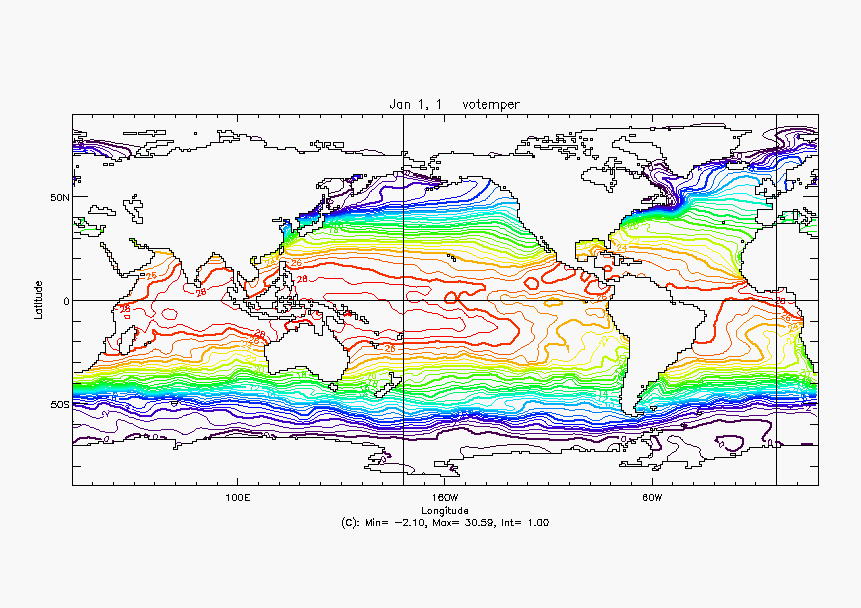
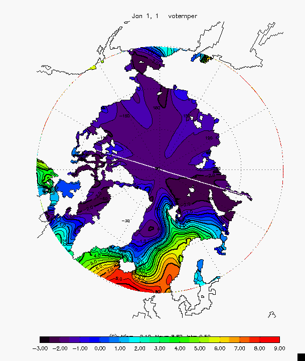
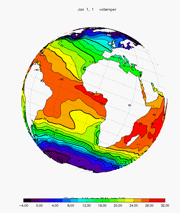
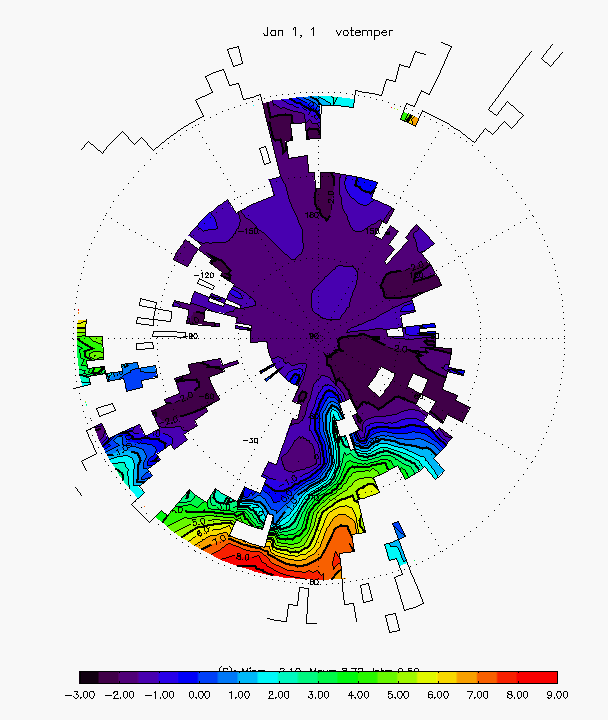
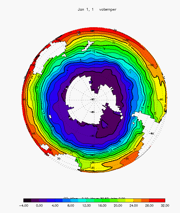
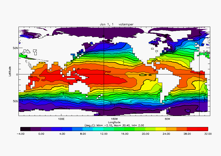
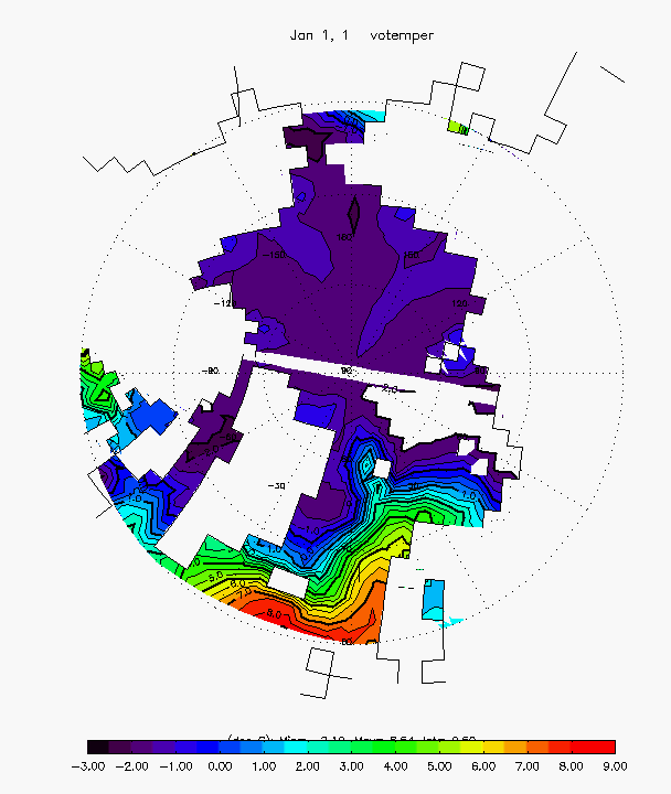
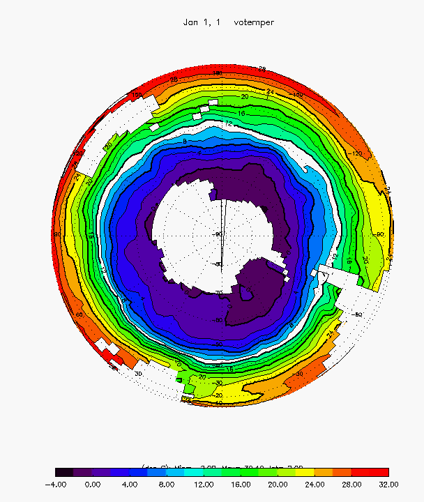
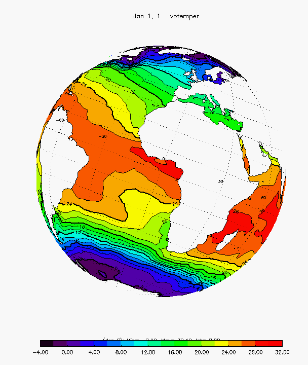
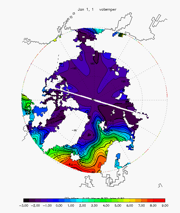
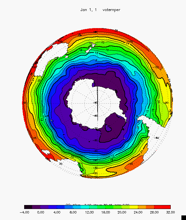
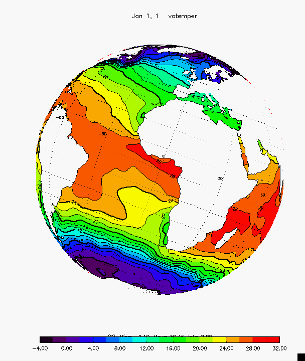
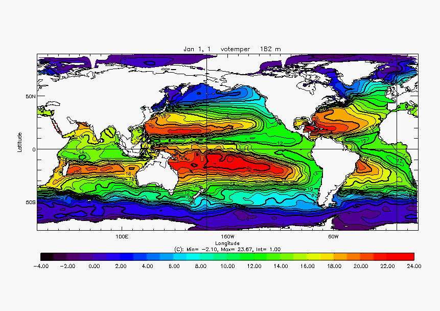
A quick presentation of horizontal plots and maps is shown in tst_plt. After loading any of the grid (for example with one of the above examples). Just try:
idl>tst_plt
Beware, the command is
tst_plt and not
@tst_plt as
tst_plt.pro is a procedure and not an
include.
See the results with
- @tst_initlev
- @tst_initorca2
- @tst_initorca05
- @tst_initlev_stride
- @tst_initorca2_stride
- @tst_initorca05_stride


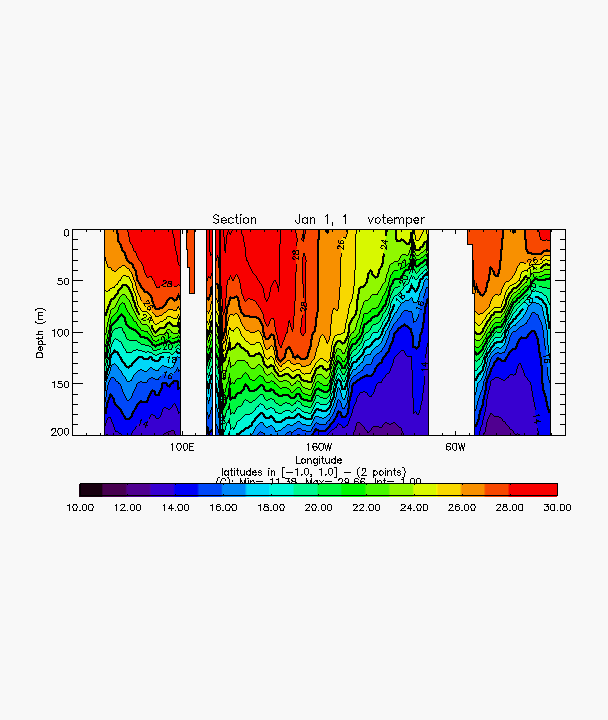
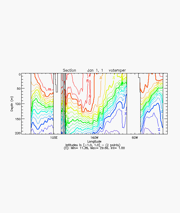
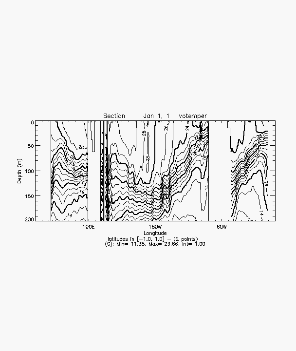
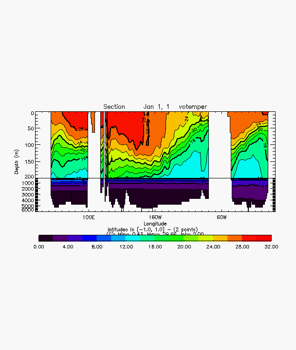
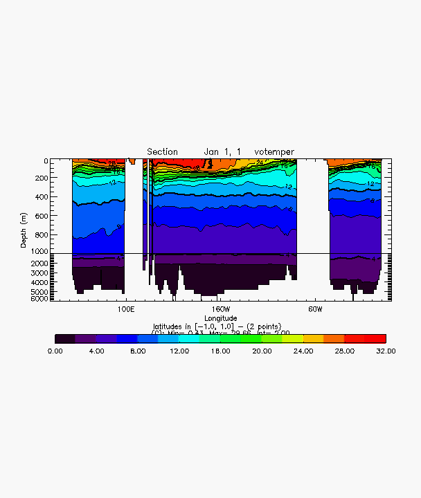
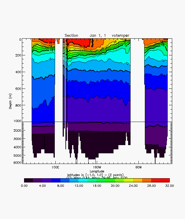
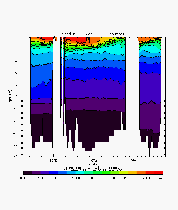
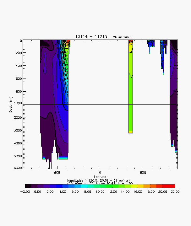
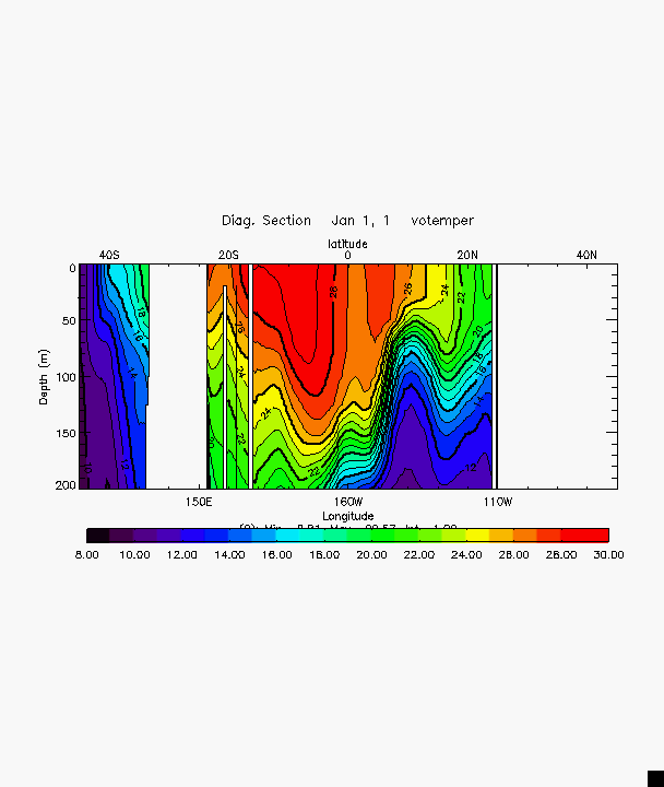
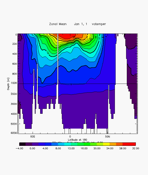
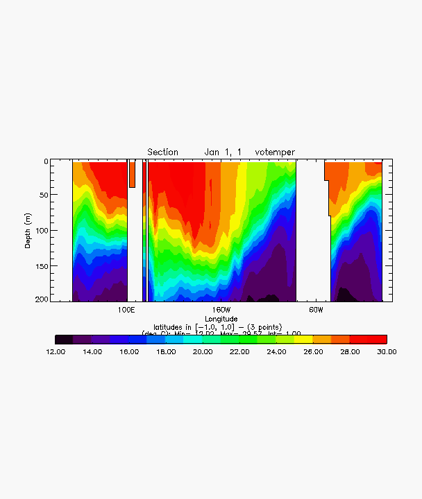
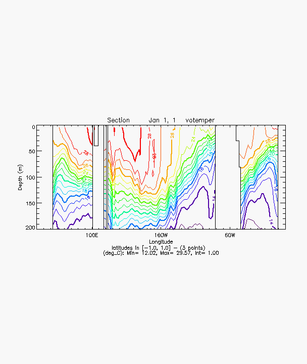
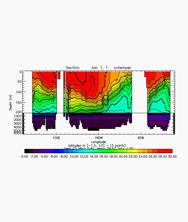
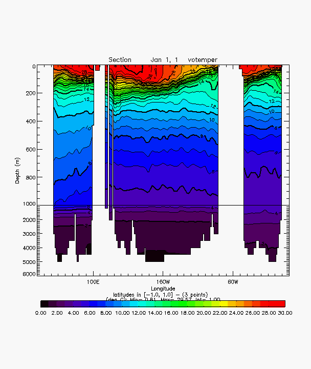
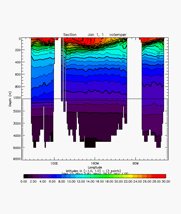
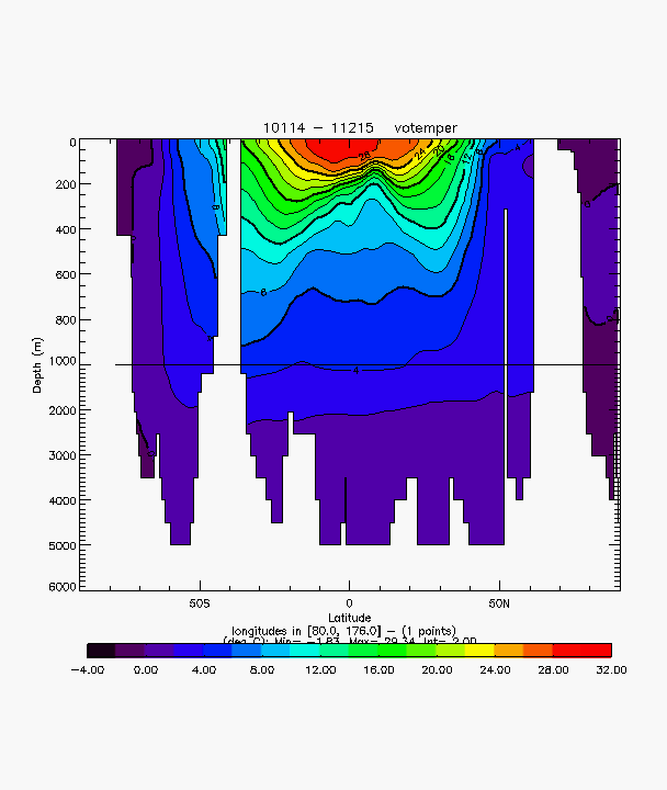
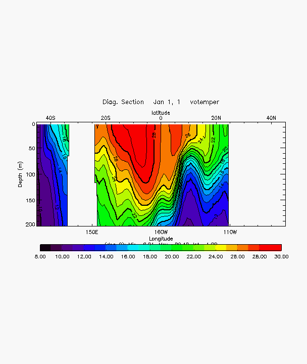
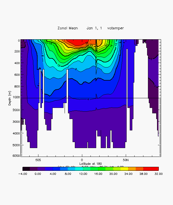
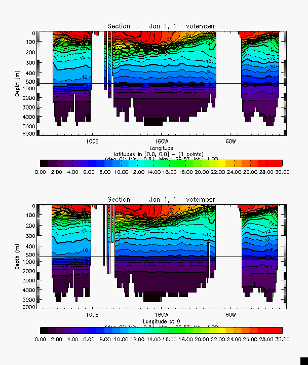
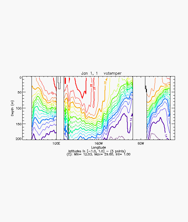
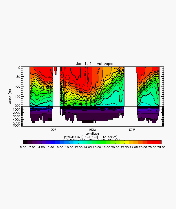
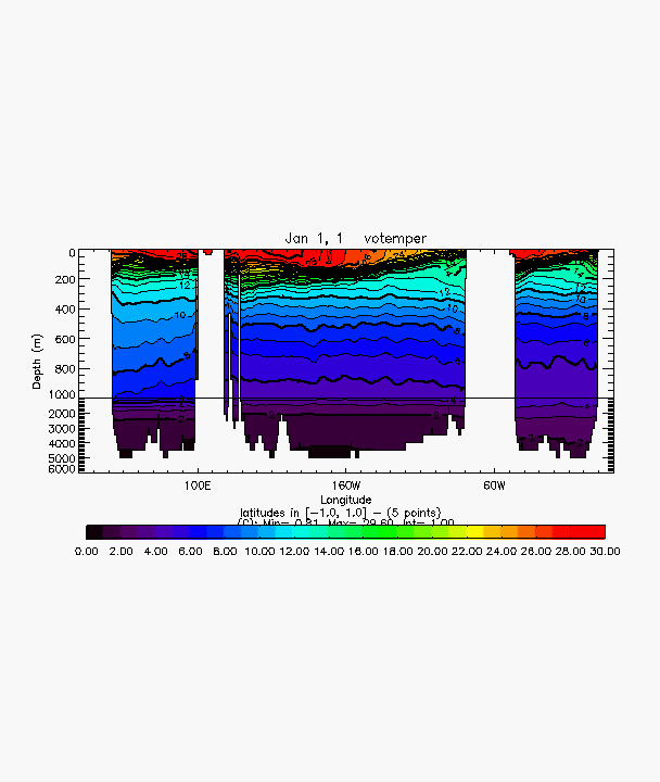
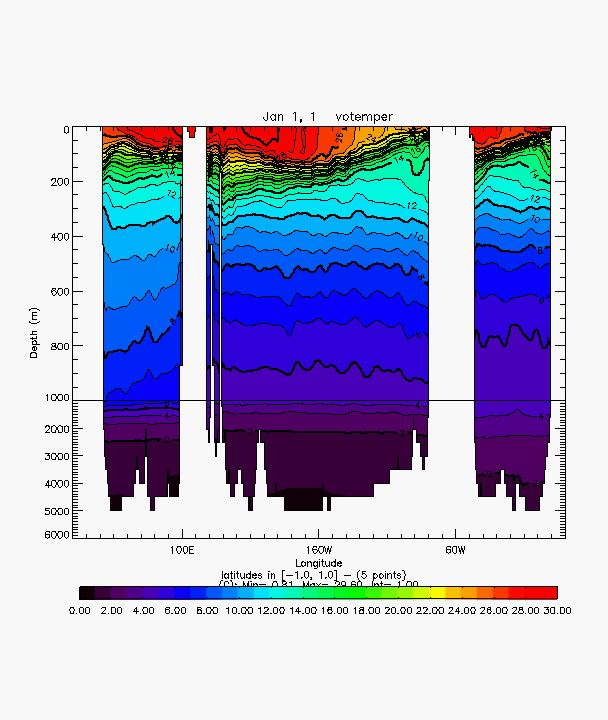
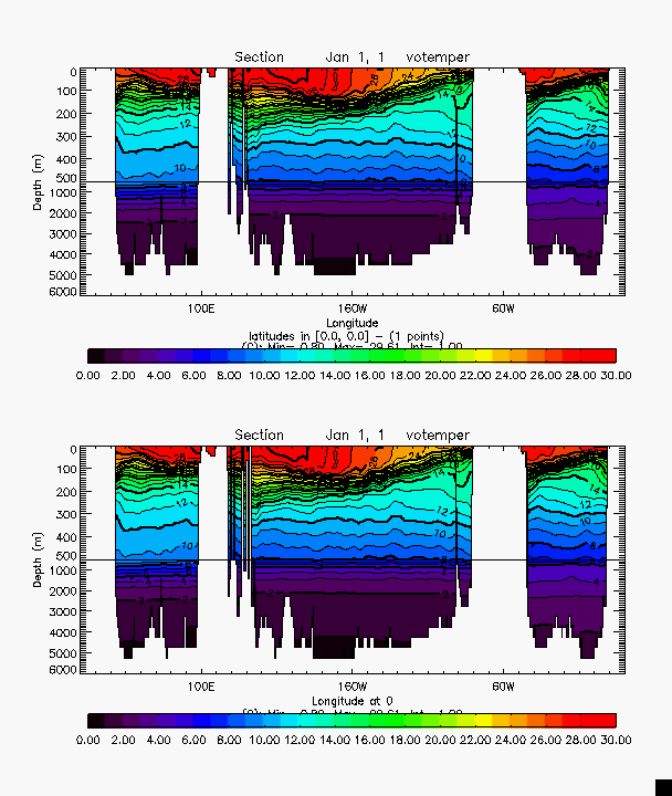
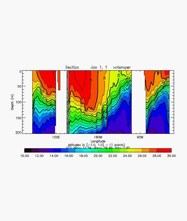
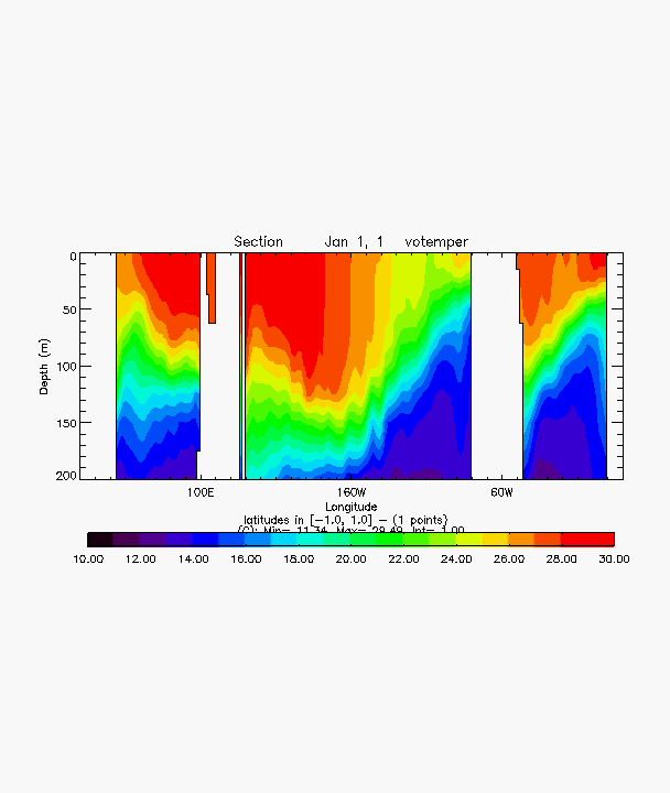
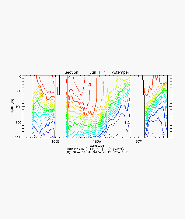
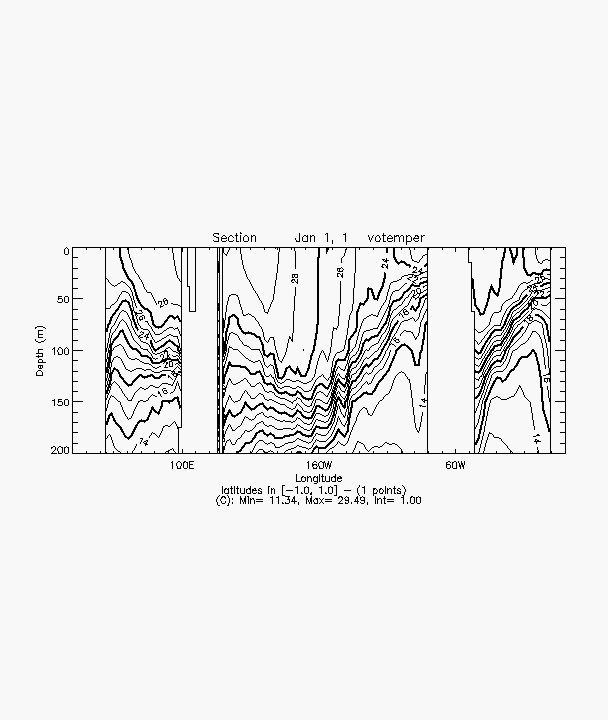
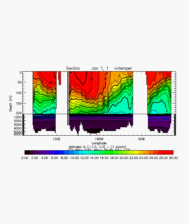
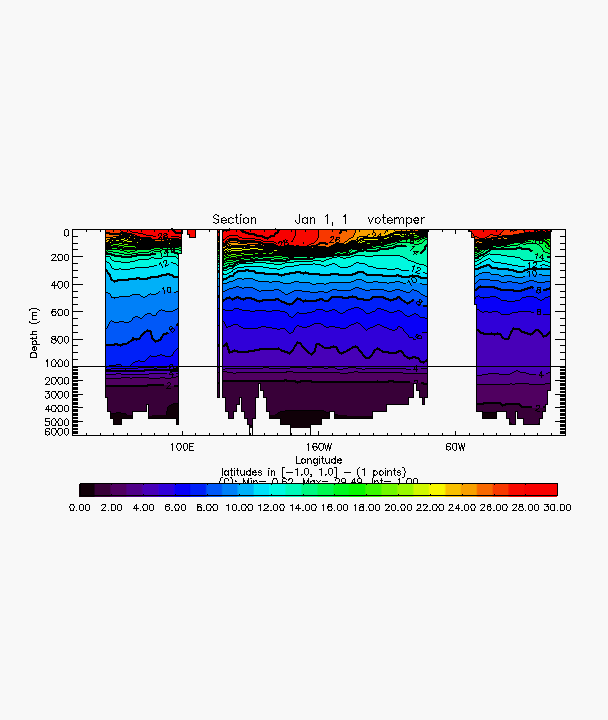
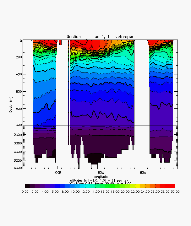
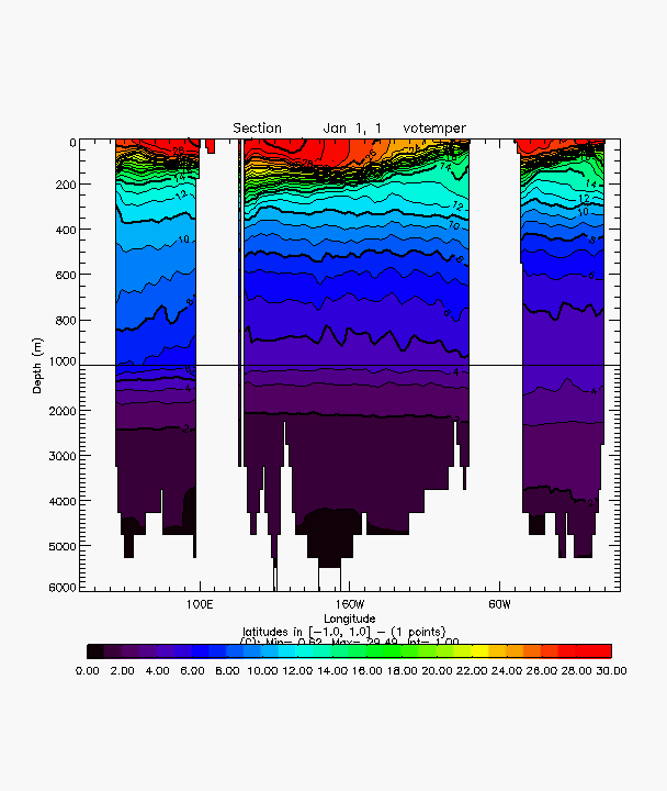
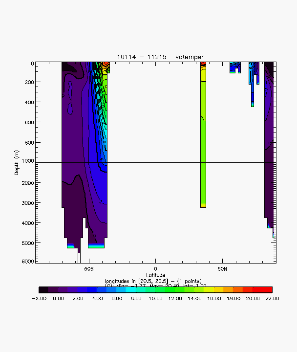
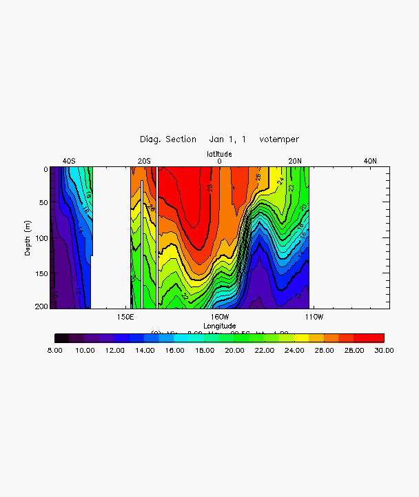
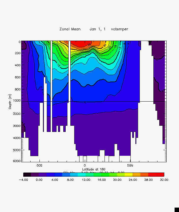
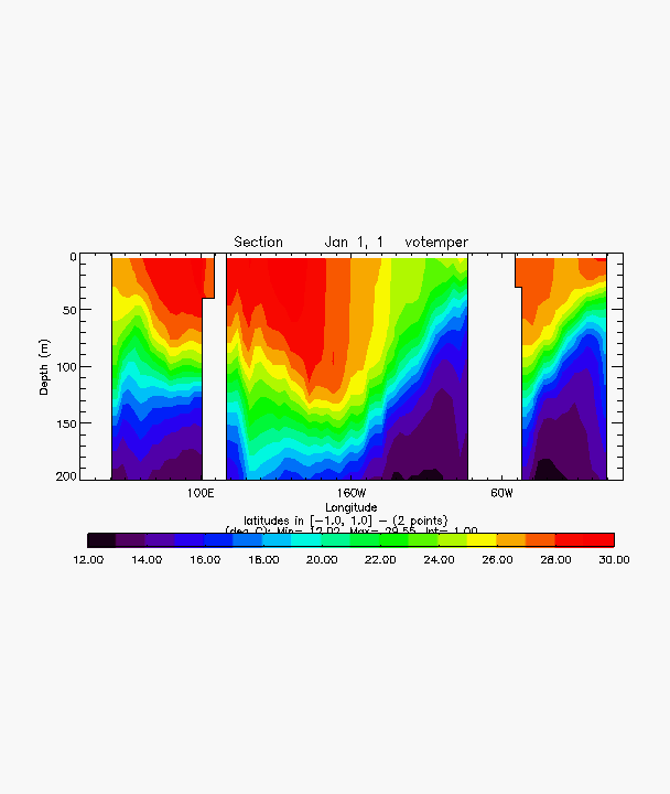
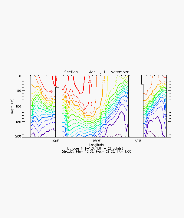
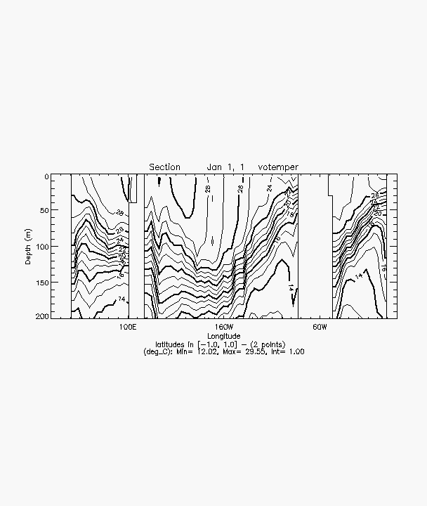
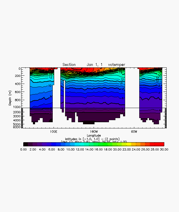
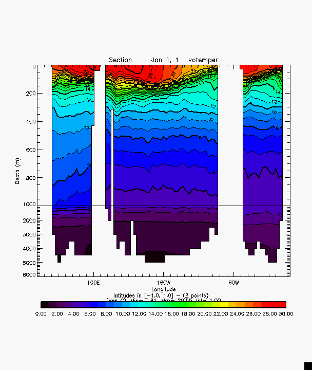
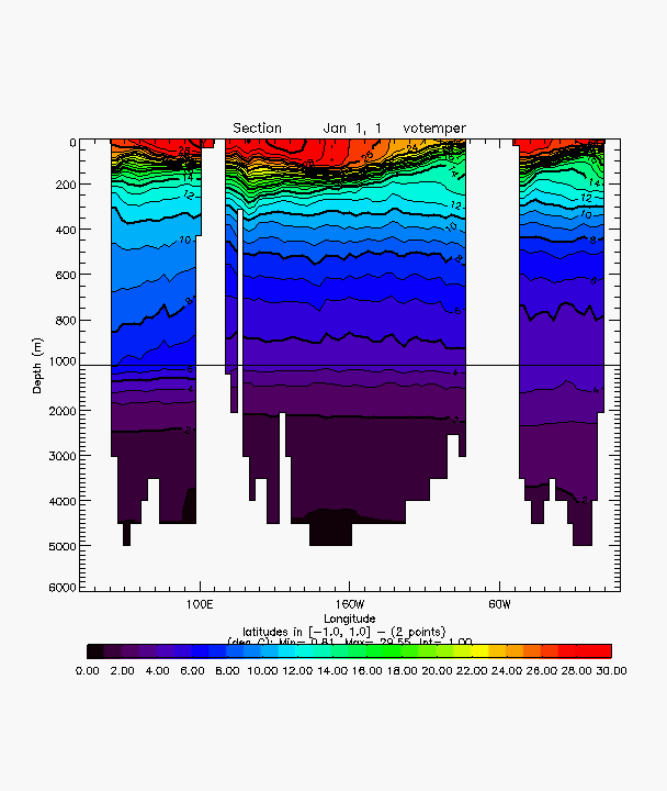
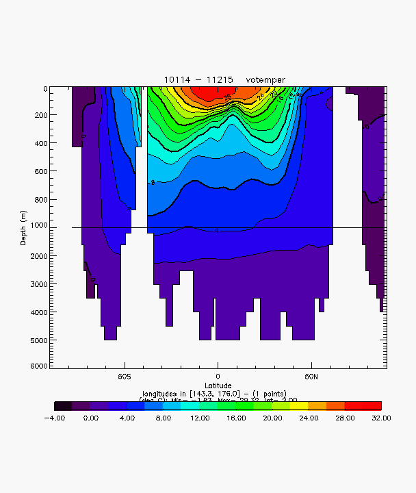
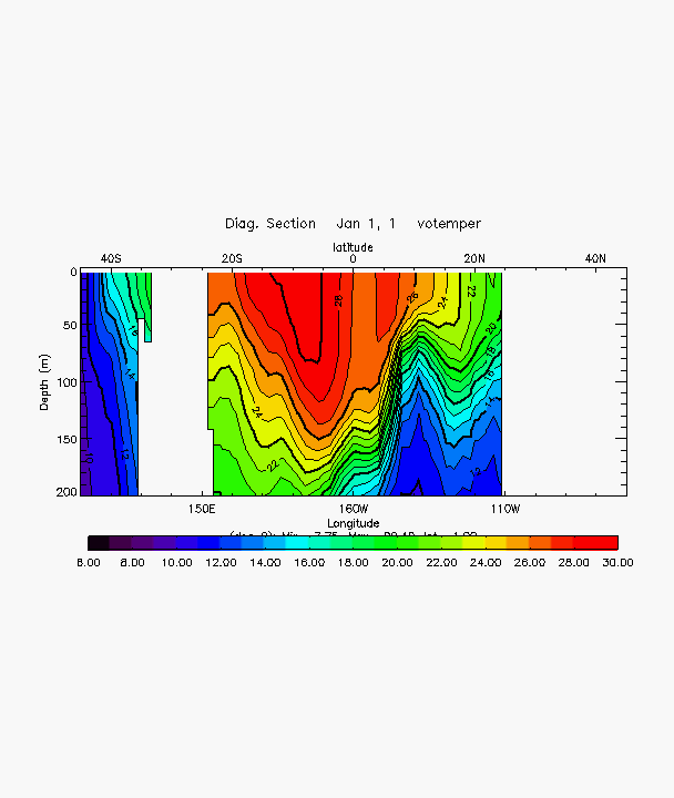
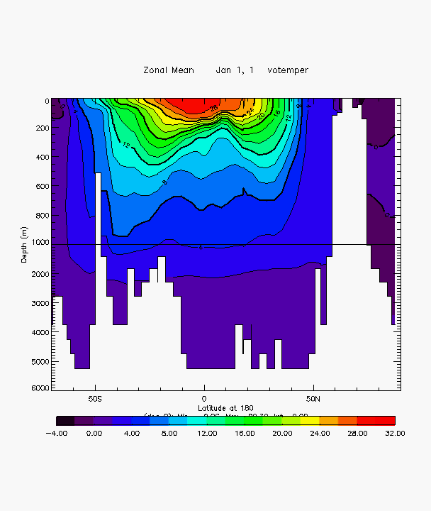
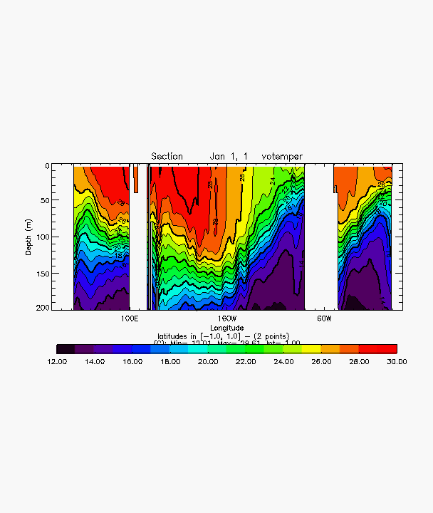
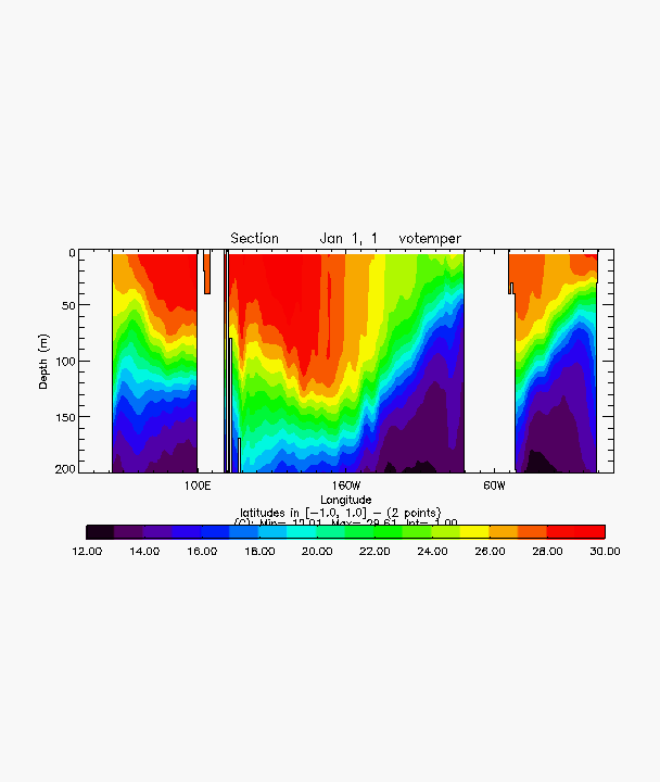
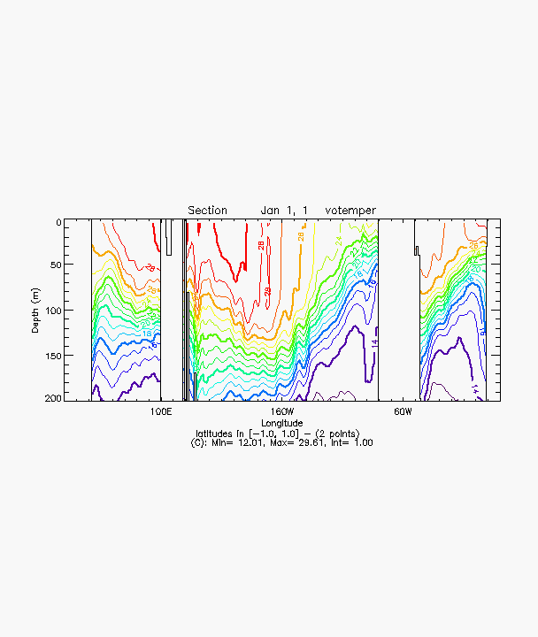
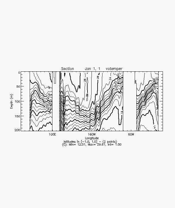
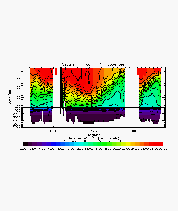
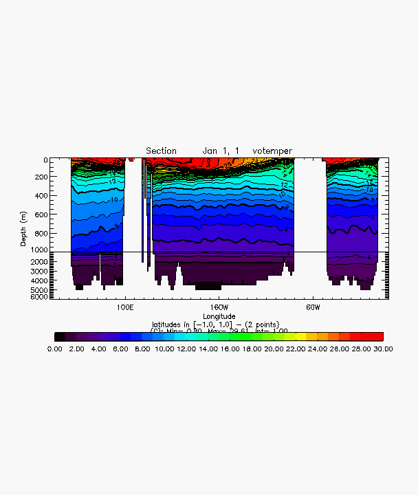
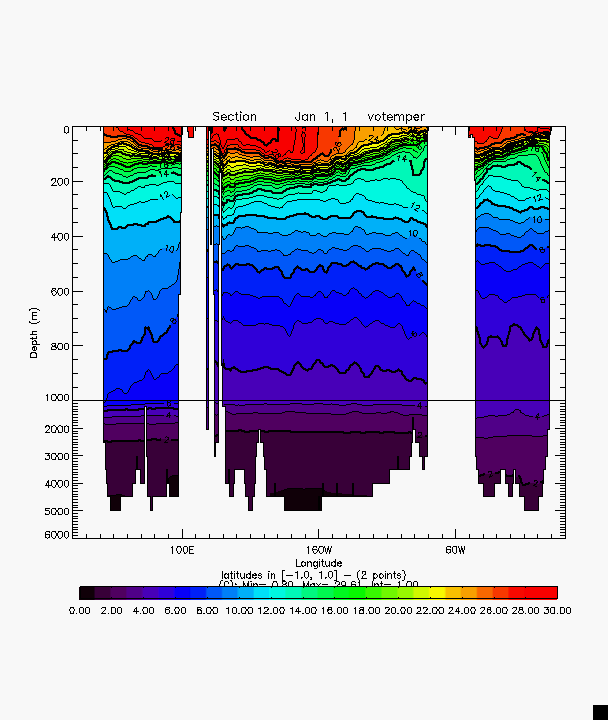
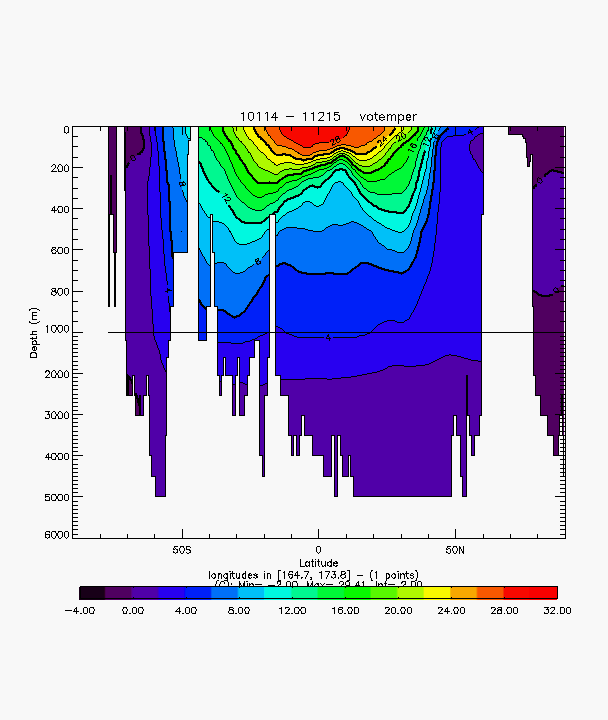
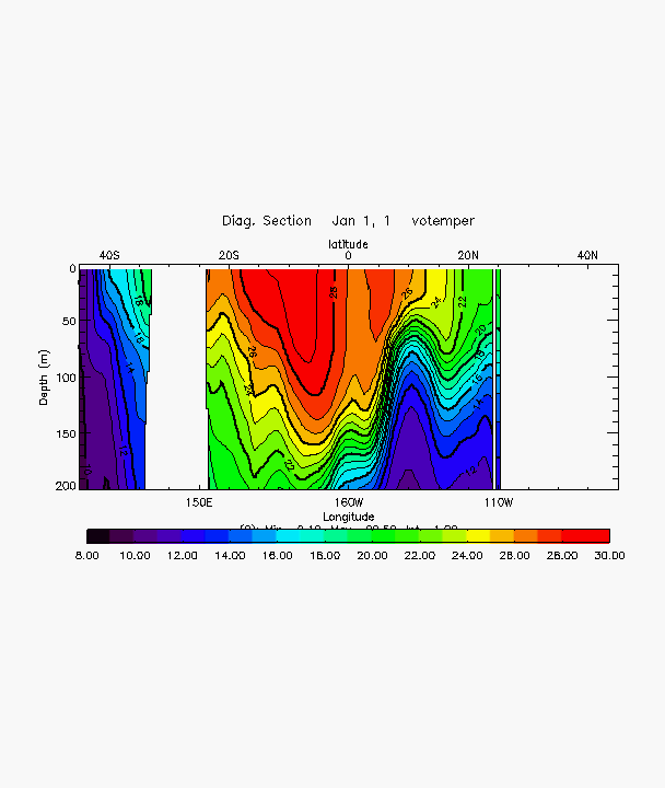
A quick presentation of vertical sections is shown in tst_pltz. After laoding any of the grid (for example with one of the above examples). Just try:
idl>tst_pltz
Beware, the command is
tst_pltz and not
@tst_pltz as
tst_pltz.pro is a procedure and not
an include.
See the results with
- @tst_initlev
- @tst_initorca2
- @tst_initorca05
- @tst_initlev_stride
- @tst_initorca2_stride
- @tst_initorca05_stride


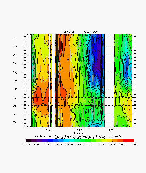
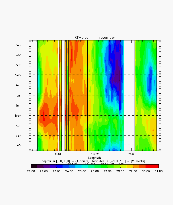
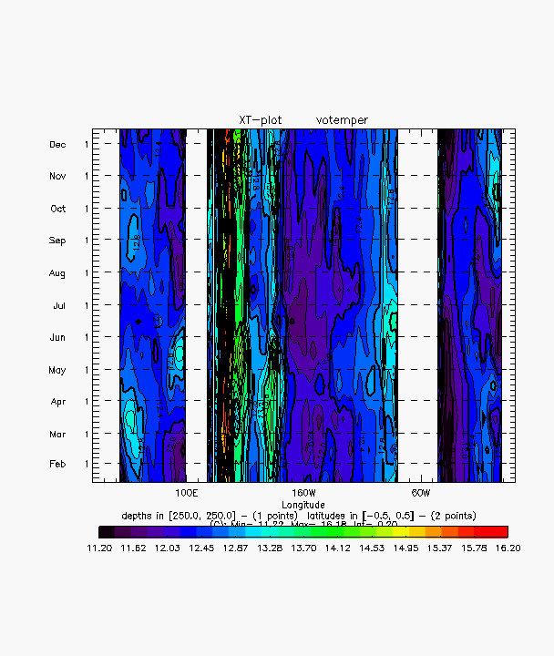
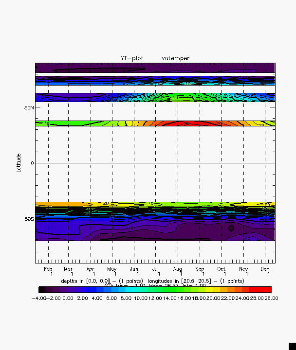
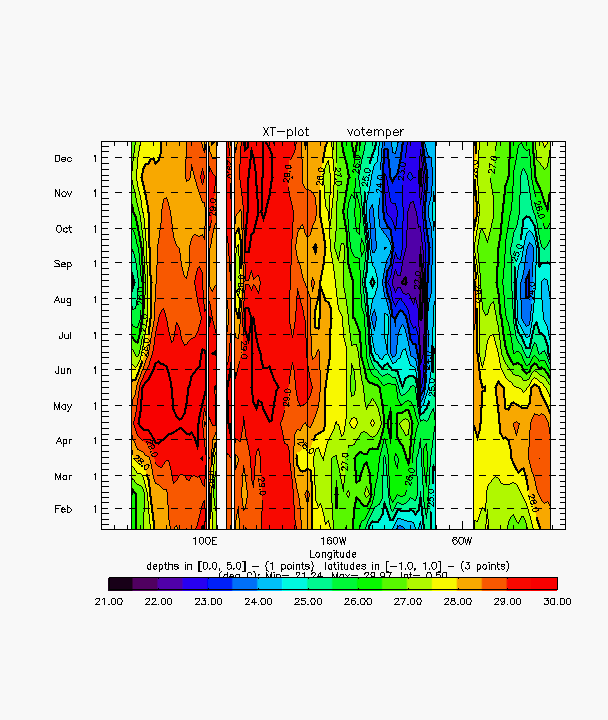
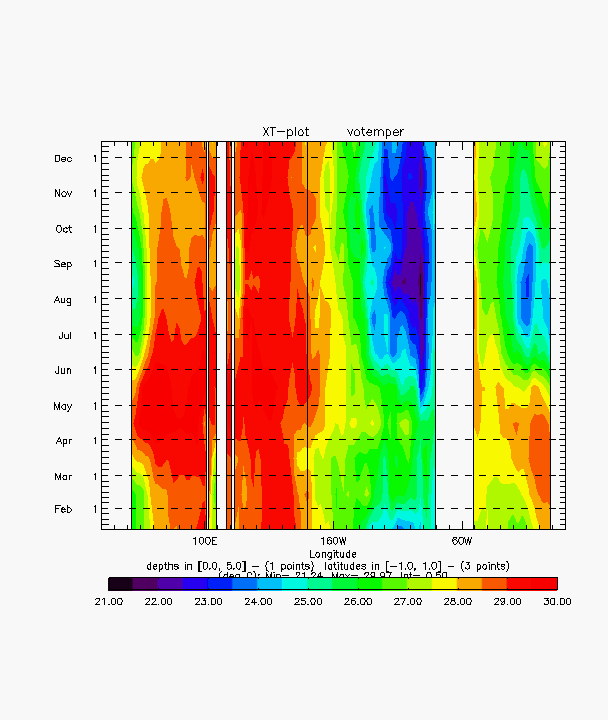
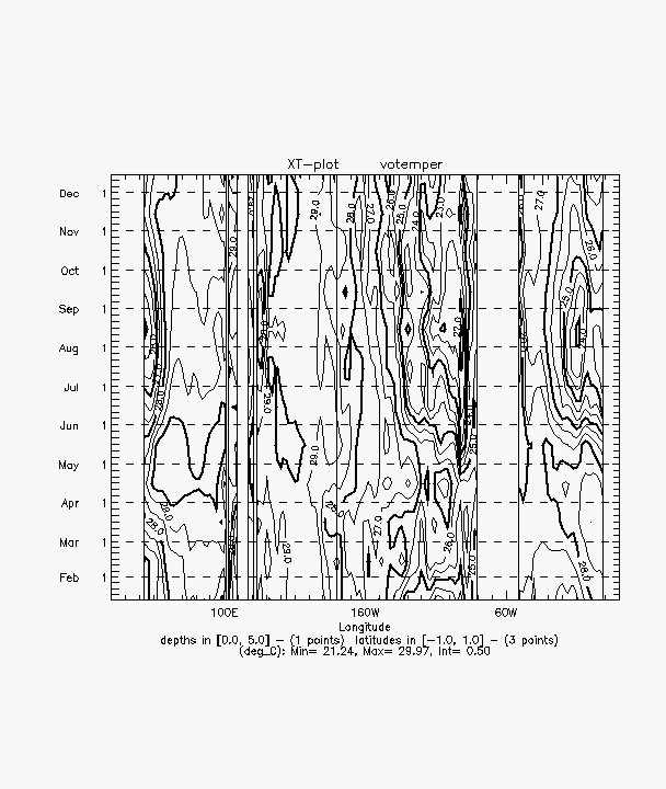
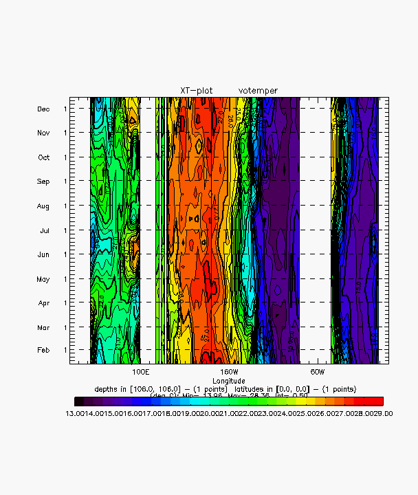
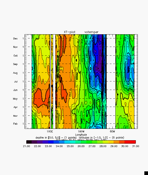
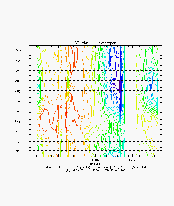
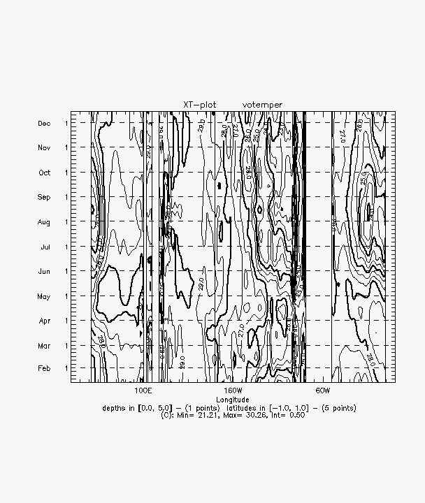
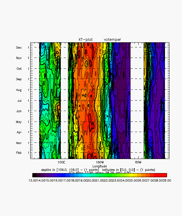
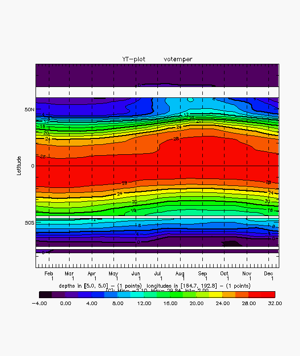
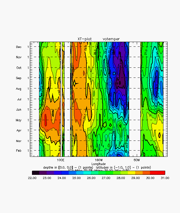
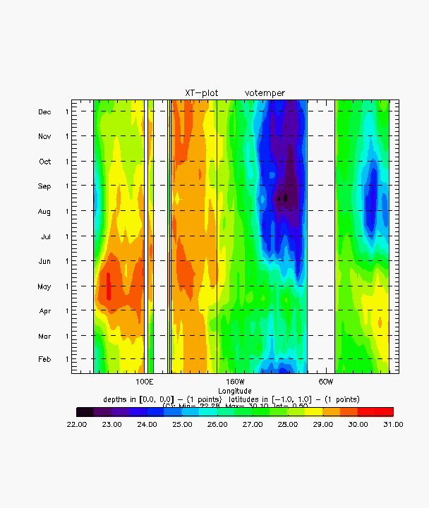
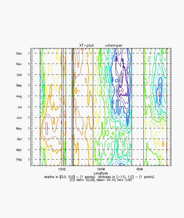
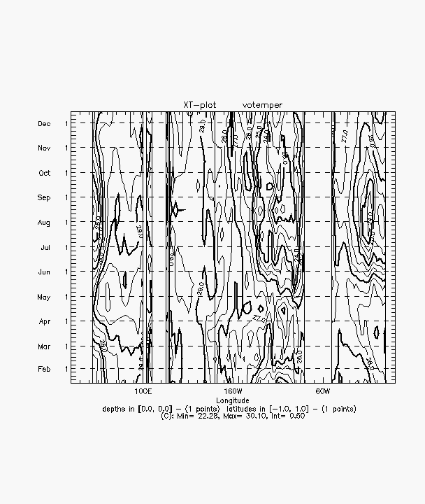
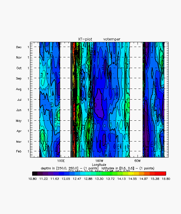
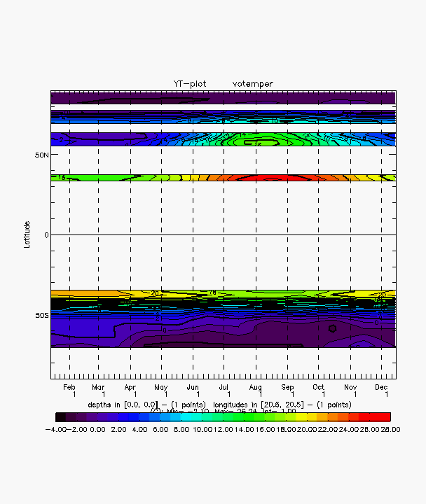
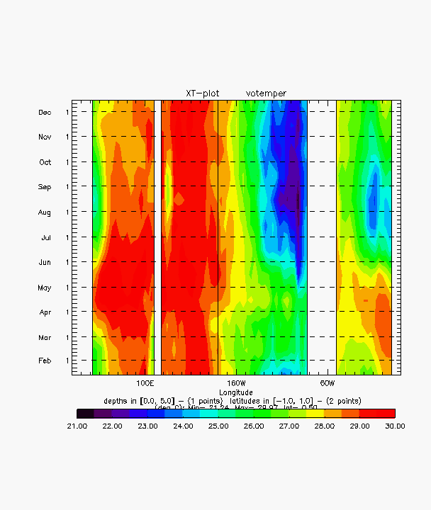
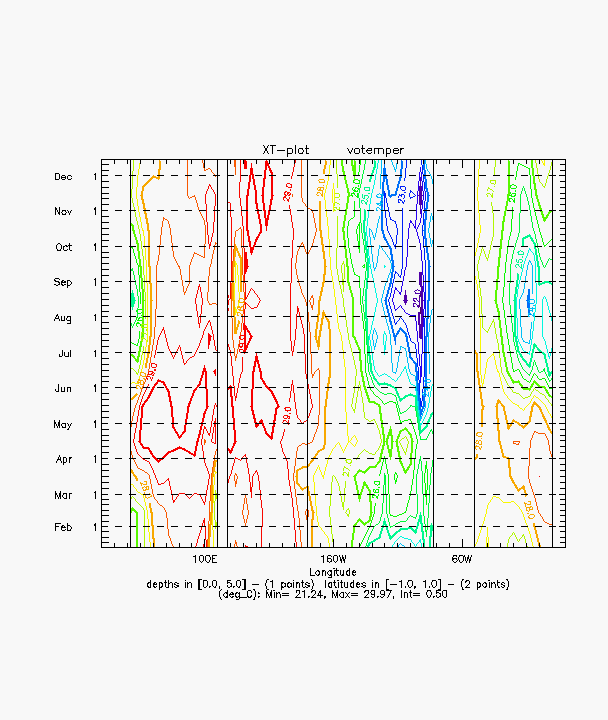
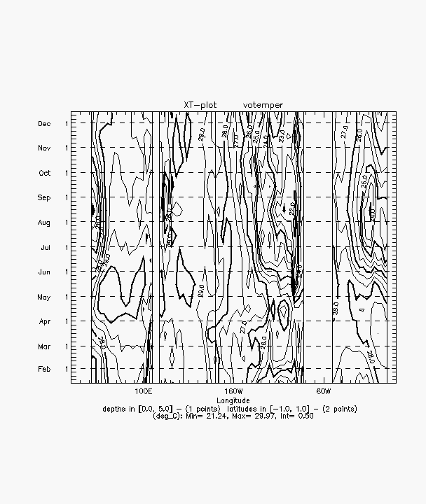
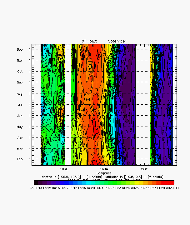
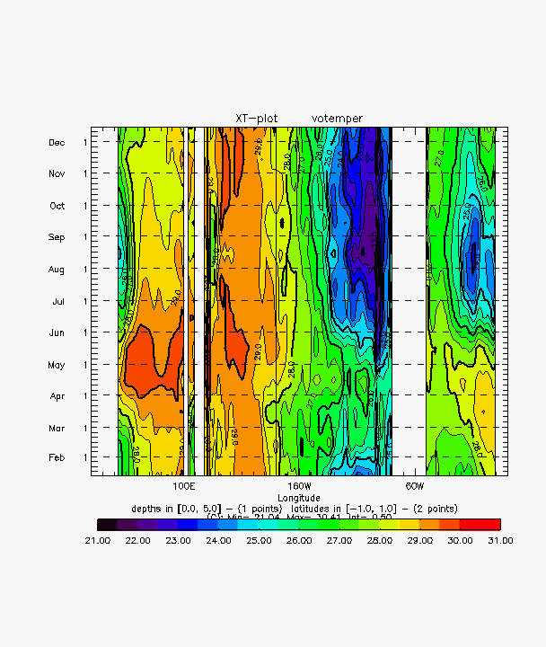
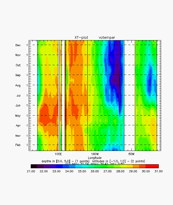
A quick presentation of hovmoellers and time series is shown in tst_pltt. After laoding any of the grid (for example with one of the above examples). Just try:
idl>tst_pltt
Beware, the command is
tst_pltt and not
@tst_pltt as
tst_pltt.pro is a procedure and not
an include.
See the results with
- @tst_initlev
- @tst_initorca2
- @tst_initorca05
- @tst_initlev_stride
- @tst_initorca2_stride
- @tst_initorca05_stride