Subsections
Eddy induced advection formulated as a skew flux
The continuous skew flux formulation
When Gent and McWilliams's [1990] diffusion is used,
an additional advection term is added. The associated velocity is the so called
eddy induced velocity, the formulation of which depends on the slopes of iso-
neutral surfaces. Contrary to the case of iso-neutral mixing, the slopes used
here are referenced to the geopotential surfaces,  (9.10)
is used in
(9.10)
is used in  -coordinate, and the sum (9.10)
+ (9.11) in
-coordinate, and the sum (9.10)
+ (9.11) in  or
or 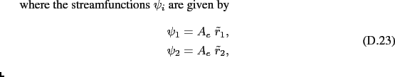 -coordinates.
The eddy induced velocity is given by:
with  the eddy induced velocity coefficient, and
 and
and
 the slopes between the iso-neutral and the geopotential surfaces.
The traditional way to implement this additional advection is to add
it to the Eulerian velocity prior to computing the tracer
advection. This is implemented if key_ traldf_eiv is set in the
default implementation, where ln_traldf_grif is set
false. This allows us to take advantage of all the advection schemes
offered for the tracers (see §5.1) and not just a  order advection scheme. This is particularly useful for passive
tracers where positivity of the advection scheme is of
paramount importance.
order advection scheme. This is particularly useful for passive
tracers where positivity of the advection scheme is of
paramount importance.
However, when ln_traldf_grif is set true, NEMO instead
implements eddy induced advection according to the so-called skew form
[Griffies, 1998]. It is based on a transformation of the advective fluxes
using the non-divergent nature of the eddy induced velocity.
For example in the (i,k) plane, the tracer advective
fluxes per unit area in 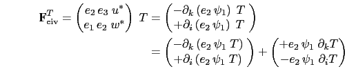 space can be
transformed as follows:
space can be
transformed as follows:
and since the eddy induced velocity field is non-divergent, we end up with the skew
form of the eddy induced advective fluxes per unit area in 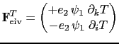 space:
 |
(D.37) |
The total fluxes per unit physical area are then
 |
(D.38) |
Note that Eq. (D.41) takes the same form whatever the
vertical coordinate, though of course the slopes
 which define the
 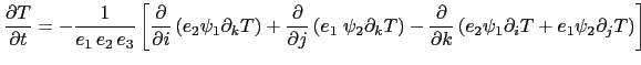 in (D.39b) are relative to geopotentials.
The tendency associated with eddy induced velocity is then simply the convergence
of the fluxes (D.40, D.41), so
in (D.39b) are relative to geopotentials.
The tendency associated with eddy induced velocity is then simply the convergence
of the fluxes (D.40, D.41), so
![$\displaystyle \frac{\partial T}{\partial t}= -\frac{1}{e_1 \, e_2 \, e_3 } \lef...
...k} \left( e_{2} \psi_1 \partial_i T + e_{1} \psi_2 \partial_j T \right) \right]$](img3943.png?doc=NEMO) |
(D.39) |
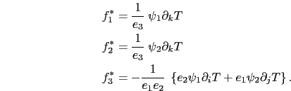
It naturally conserves the tracer content, as it is expressed in flux
form. Since it has the same divergence as the advective form it also
preserves the tracer variance.
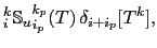
The skew fluxes in (D.41, D.40), like the off-diagonal terms
(D.3, D.4) of the small angle diffusion tensor, are best
expressed in terms of the triad slopes, as in Fig. D.1
and Eqs (D.6, D.7); but now in terms of the triad slopes
 relative to geopotentials instead of the
 relative to coordinate surfaces. The discrete form of
(D.40) using the slopes (D.8) and
defining
relative to coordinate surfaces. The discrete form of
(D.40) using the slopes (D.8) and
defining  at
at 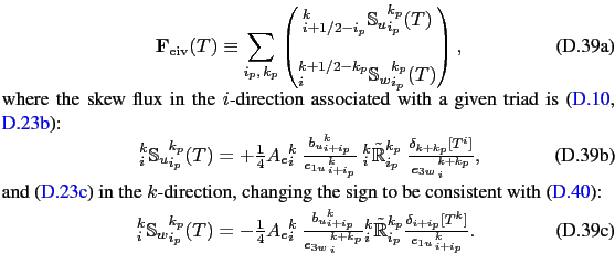 -points is then given by:
Such a discretisation is consistent with the iso-neutral
operator as it uses the same definition for the slopes. It also
ensures the following two key properties.
The discretization conserves tracer variance,  it does not
include a diffusive component but is a `pure' advection term. This can
be seen
by considering the
fluxes associated with a given triad slope
it does not
include a diffusive component but is a `pure' advection term. This can
be seen
by considering the
fluxes associated with a given triad slope
 . For, following
§D.2.5 and (D.16), the
associated horizontal skew-flux
. For, following
§D.2.5 and (D.16), the
associated horizontal skew-flux
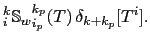
 drives a net rate of change of variance, summed over the two
 -points
 and
and
 , of
, of
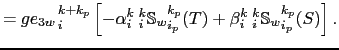
![$\displaystyle _i^k{\mathbb{S}_u}_{i_p}^{k_p} (T)\,\delta_{i+ i_p}[T^k],$](img3955.png?doc=NEMO) |
(D.41) |
while the associated vertical skew-flux gives a variance change summed over the
 -points
 (above) and
 (below) of
![$\displaystyle _i^k{\mathbb{S}_w}_{i_p}^{k_p} (T) \,\delta_{k+ k_p}[T^i].$](img3959.png?doc=NEMO) |
(D.42) |
Inspection of the definitions (D.43b, D.43c)
shows that these two variance changes (D.44, D.45)
sum to zero. Hence the two fluxes associated with each triad make no
net contribution to the variance budget.
The vertical density flux associated with the vertical skew-flux
always has the same sign as the vertical density gradient; thus, so
long as the fluid is stable (the vertical density gradient is
negative) the vertical density flux is negative (downward) and hence
reduces the gravitational PE.
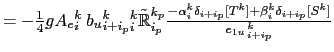
For the change in gravitational PE driven by the 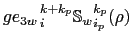 -flux is
using the definition of the triad slope
 ,
(D.8) to express
,
(D.8) to express
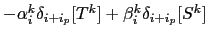
![$ -\alpha _i^k\delta_{i+ i_p}[T^k]+
\beta_i^k\delta_{i+ i_p}[S^k]$](img3967.png?doc=NEMO) in terms of
in terms of
![$ -\alpha_i^k \delta_{k+
k_p}[T^i]+ \beta_i^k\delta_{k+ k_p}[S^i]$](img3968.png?doc=NEMO) .
.
Where the coordinates slope, the 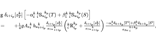 -flux gives a PE change
(using (D.43b)) and so the total PE change
(D.46) + (D.47) associated with the triad fluxes is
Where the fluid is stable, with
![$ -\alpha_i^k \delta_{k+ k_p}[T^i]+
\beta_i^k\delta_{k+ k_p}[S^i]<0$](img3972.png?doc=NEMO) , this PE change is negative.
, this PE change is negative.
Treatment of the triads at the boundaries
Triad slopes R used for the calculation of the eddy-induced skew-fluxes
are masked at the boundaries in exactly the same way as are the triad
slopes R used for the iso-neutral diffusive fluxes, as
described in §D.2.8 and
Fig. D.3. Thus surface layer triads
 and
and
 are
masked, and both near bottom triad slopes
are
masked, and both near bottom triad slopes
 and
and
 are masked when either of the
 or
or  tracer points is masked, i.e. the
 -point is masked. The namelist parameter ln_botmix_grif has
no effect on the eddy-induced skew-fluxes.
-point is masked. The namelist parameter ln_botmix_grif has
no effect on the eddy-induced skew-fluxes.
Limiting of the slopes within the interior
Presently, the iso-neutral slopes
 relative
to geopotentials are limited to be less than
relative
to geopotentials are limited to be less than  , exactly as in
calculating the iso-neutral diffusion, §D.2.9. Each
individual triad R is so limited.
, exactly as in
calculating the iso-neutral diffusion, §D.2.9. Each
individual triad R is so limited.
Tapering within the surface mixed layer
The slopes
 relative to
geopotentials (and thus the individual triads R) are always tapered linearly from their value immediately below the mixed layer to zero at the
surface (D.32a), as described in §D.2.10. This is
option (c) of Fig. 9.2. This linear tapering for the
slopes used to calculate the eddy-induced fluxes is
unaffected by the value of ln_triad_iso.
relative to
geopotentials (and thus the individual triads R) are always tapered linearly from their value immediately below the mixed layer to zero at the
surface (D.32a), as described in §D.2.10. This is
option (c) of Fig. 9.2. This linear tapering for the
slopes used to calculate the eddy-induced fluxes is
unaffected by the value of ln_triad_iso.
The justification for this linear slope tapering is that, for  that is constant or varies only in the horizontal (the most commonly
used options in NEMO: see §9.1), it is
equivalent to a horizontal eiv (eddy-induced velocity) that is uniform
within the mixed layer (D.39a). This ensures that the
eiv velocities do not restratify the mixed layer [Danabasoglu et al., 2008, Tréguier et al., 1997]. Equivantly, in terms
of the skew-flux formulation we use here, the
linear slope tapering within the mixed-layer gives a linearly varying
vertical flux, and so a tracer convergence uniform in depth (the
horizontal flux convergence is relatively insignificant within the mixed-layer).
that is constant or varies only in the horizontal (the most commonly
used options in NEMO: see §9.1), it is
equivalent to a horizontal eiv (eddy-induced velocity) that is uniform
within the mixed layer (D.39a). This ensures that the
eiv velocities do not restratify the mixed layer [Danabasoglu et al., 2008, Tréguier et al., 1997]. Equivantly, in terms
of the skew-flux formulation we use here, the
linear slope tapering within the mixed-layer gives a linearly varying
vertical flux, and so a tracer convergence uniform in depth (the
horizontal flux convergence is relatively insignificant within the mixed-layer).
Streamfunction diagnostics
Where the namelist parameter ln_traldf_gdia=true, diagnosed
mean eddy-induced velocities are output. Each time step,
streamfunctions are calculated in the  -
- and
and  -
- planes at
 (integer +1/2
  , integer
  , integer +1/2
  ) and
) and  (integer
  , integer +1/2
  , integer +1/2
  ) points (see Table
4.1) respectively. We follow [Griffies, 2004] and
calculate the streamfunction at a given
) points (see Table
4.1) respectively. We follow [Griffies, 2004] and
calculate the streamfunction at a given  -point from the
surrounding four triads according to:
-point from the
surrounding four triads according to:
 |
(D.44) |
The streamfunction  is calculated similarly at
 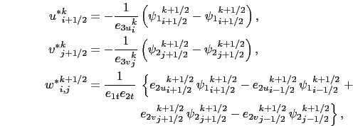 points.
The eddy-induced velocities are then calculated from the
straightforward discretisation of (D.39a):
points.
The eddy-induced velocities are then calculated from the
straightforward discretisation of (D.39a):
Gurvan Madec and the NEMO Team
NEMO European Consortium2016-11-22
 from
(D.43c), gives
from
(D.43c), gives![$\displaystyle =-\quarter g{A_e}_i^k{\: }{b_u}_{i+i_p}^k {_i^k\tilde{\mathbb{R}}...
...ta_{i+ i_p}[T^k]+ \beta_i^k\delta_{i+ i_p}[S^k]} { {e_{1u}}_{\,i + i_p}^{\,k} }$](img3964.png?doc=NEMO)
![\begin{multline}
g \delta_{i+i_p}[z_T^k]
\left[
-\alpha _i^k {\:}_i^k {\mathb...
...[T^i]+ \beta_i^k\delta_{k+ k_p}[S^i]} {{e_{3w}}_{\,i}^{\,k+k_p}},
\end{multline}](img3970.png?doc=NEMO)